Slowing down, heating and current drive

Download notebook View on GitHubRun when the site was built.

Follow the fast ions from their birth until they join the thermal plasma: how their energy splits between electrons and ions, the fast-ion density and pressure they build up, and the current they drive.

slow_down uses classical (Stix) slowing down on the flux surface where each ion is born, with the local electron density and temperature: a fast ion loses speed as dv/dt = -(v^3 + v_c^3) / (tau_s v^2), with the Spitzer slowing-down time on the electrons tau_s and the critical velocity v_c, where the electron and ion drags are equal (Stix, Plasma Phys. 14, 367, 1972).

import matplotlib.pyplot as plt
import numpy as np
from plasmacoll.constants import ATOMIC_MASS, ELEMENTARY_CHARGE
from scipy.integrate import quad

import freeofcharge as foc
from freeofcharge.slowing_down import (
    critical_velocity,
    ion_heating_fraction,
    slowing_down_time,
)

ne, te = 1e20, 2e4
densities = [0.96 * ne, 0.02 * ne]  # D and He
masses = [2 * ATOMIC_MASS, 4 * ATOMIC_MASS]
charges = [1, 2]
mass_b = 2 * ATOMIC_MASS  # a deuterium beam

v_c = float(critical_velocity(ne, te, densities, masses, charges))
critical_energy = 0.5 * mass_b * v_c**2 / ELEMENTARY_CHARGE
# Stix's form E_c = 14.8 T_e A_b (sum_j n_j Z_j^2 / (n_e A_j))^(2/3)
stix = 14.8 * te * 2 * ((densities[0] * 1 / 2 + densities[1] * 4 / 4) / ne) ** (2 / 3)
tau_s = float(slowing_down_time(mass_b, 1, ne, te))
print(
    f"critical energy {critical_energy / 1e3:.1f} keV (Stix's 14.8 T_e form: {stix / 1e3:.1f} keV)"
)
print(f"slowing-down time on the electrons: {tau_s:.2f} s")
assert abs(critical_energy / stix - 1) < 0.01

critical energy 372.1 keV (Stix's 14.8 T_e form: 372.9 keV)
slowing-down time on the electrons: 1.99 s

Above the critical energy E_c a fast ion heats mostly the electrons, below it mostly the ions. The share of its energy that goes to the ions over its whole slowing down is (1/x) int_0^x dy / (1 + y^(3/2)) with x = E_0 / E_c; freeofcharge evaluates it in closed form, which matches a direct quadrature. A 1 MeV deuteron born at the centre, at 20 keV, gives almost half of its energy to the ions:

ratio = np.geomspace(0.1, 30, 60)
share = np.asarray(ion_heating_fraction(ratio))
for x in (0.5, 1.0, 3.0, 10.0):
    direct = quad(lambda y: 1 / (1 + y**1.5), 0, x)[0] / x
    assert abs(float(ion_heating_fraction(x)) - direct) < 1e-9

x_beam = 1e6 / critical_energy
fig, ax = plt.subplots(figsize=(5.5, 3.5), layout="constrained")
ax.semilogx(ratio, share, label="to the ions")
ax.semilogx(ratio, 1 - share, label="to the electrons")
ax.axvline(x_beam, color="0.5", linestyle=":", label="1 MeV D at 20 keV")
ax.set_xlabel("E_0 / E_c")
ax.set_ylabel("share of the fast ion's energy")
ax.legend()
plt.show()
print(f"1 MeV: {100 * float(ion_heating_fraction(x_beam)):.0f} % to the ions")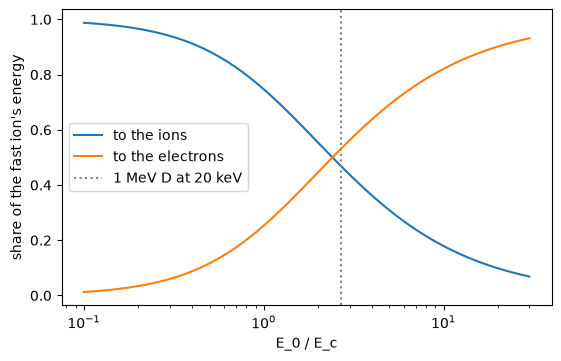

1 MeV: 47 % to the ions

Heating and current profiles

slow_down(deposition, plasma, surfaces) adds up the births of a deposition, shell by shell, in steady state: the power to the electrons and to the ions, the fast-ion density (birth rate times slowing-down time), the pressure (two thirds of the energy density) and the parallel current of the fast ions. The fast ions’ pitch relaxes by pitch-angle scattering on the ions as they slow down. Their current is shielded by the electrons, j = j_fast (1 - Z_b / Z_eff (1 - G)), with a trapped-electron correction G that grows with the inverse aspect ratio. Every watt the beam deposits ends up in the electrons or the ions. Most fast ions are born off axis, where the electrons are colder and E_c lower, so over the whole beam the ions get only about a third:

equilibrium = foc.Equilibrium.solovev(6.2, 1.8, 1.7, 5.3, wall_psi_n=1.3)
plasma = foc.Plasma.parabolic(ne, te, ions={"D": (2, 1, 0.96), "He": (4, 2, 0.02)})
rho_edges = np.linspace(0.0, 1.0, 21)
surfaces = equilibrium.flux_surfaces(rho_edges)

steady = {}
for sense in (1, -1):
    origin, direction = foc.tangential_injection(5.3, 12.0, sense=sense)
    beam = foc.NeutralBeam.gaussian(
        origin,
        direction,
        1.0e6,
        16.5e6,
        width=0.3,
        divergence=0.005,
        markers=500,
        seed=1,
    )
    deposition = foc.deposit(
        beam,
        equilibrium,
        plasma,
        step=0.03,
        births_per_marker=2,
        rho_edges=rho_edges,
        seed=2,
    )
    steady[sense] = foc.slow_down(deposition, plasma, surfaces)
    heating = steady[sense].electron_heating.sum() + steady[sense].ion_heating.sum()
    assert abs(heating / deposition.absorbed_power - 1) < 1e-9

co = steady[1]
print(
    f"to the electrons {co.electron_heating.sum() / 1e6:.2f} MW, to the ions {co.ion_heating.sum() / 1e6:.2f} MW"
)
print(
    f"driven current {co.driven_current / 1e6:.2f} MA, fast-ion energy {co.stored_energy / 1e6:.2f} MJ"
)
print(f"counter-injection drives {steady[-1].driven_current / 1e6:.2f} MA")
assert co.driven_current > 0 > steady[-1].driven_current
assert abs(co.driven_current / -steady[-1].driven_current - 1) < 0.05

fig, (ax0, ax1, ax2) = plt.subplots(1, 3, figsize=(13, 3.5), layout="constrained")
ax0.plot(
    surfaces.rho, co.electron_heating / surfaces.volume / 1e3, "o-", label="electrons"
)
ax0.plot(surfaces.rho, co.ion_heating / surfaces.volume / 1e3, "s-", label="ions")
ax0.set_ylabel("heating [kW/m^3]")
ax0.legend()
ax1.plot(surfaces.rho, co.fast_ion_pressure / 1e3, "o-")
ax1.set_ylabel("fast-ion pressure [kPa]")
ax2.plot(surfaces.rho, co.fast_ion_current_density / 1e3, "o-", label="fast ions")
ax2.plot(surfaces.rho, co.current_density / 1e3, "s-", label="with electron shielding")
ax2.set_ylabel("current density [kA/m^2]")
ax2.legend()
for ax in (ax0, ax1, ax2):
    ax.set_xlabel("rho")
plt.show()

to the electrons 10.86 MW, to the ions 5.62 MW
driven current 0.97 MA, fast-ion energy 6.32 MJ
counter-injection drives -0.96 MA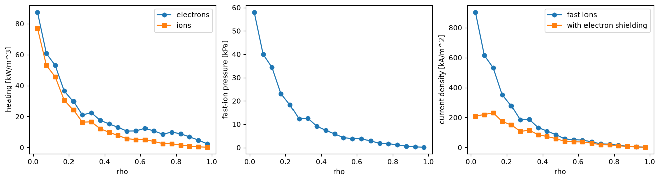

Reversing the beam (sense=-1) reverses the current: the births lie on the mirror image of the same path, so the profiles agree within the sampling noise. steady.to_dataset() returns all profiles as an xarray dataset for plasma-plots.

What the model leaves out: the orbit width (every ion stays on its birth surface), prompt losses, charge-exchange losses of fast ions and anything 3D. Two parts are still to be checked against their sources: the trapped-electron correction (a large-aspect-ratio fit attributed to Start and Cordey, see trapped_electron_correction) and the exponent of the pitch relaxation, derived from the collision rates rather than taken from Gaffey (1976).