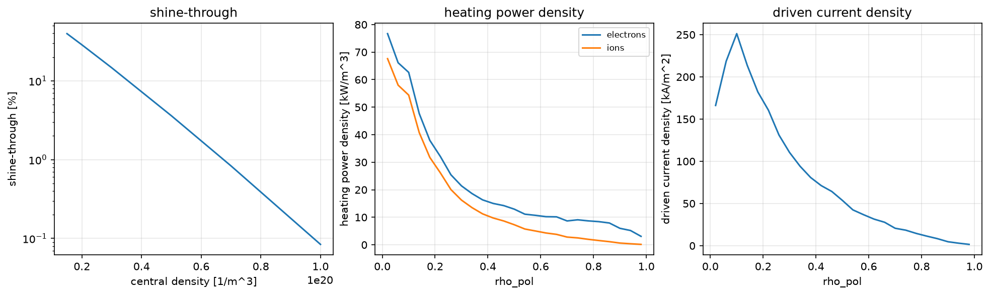
A 1 MeV deuterium beam in an ITER-like plasma: shine-through, heating, current.

One 16.5 MW beam of 1 MeV atoms, tangent to R = 5.3 m, enters a Solov’ev equilibrium of ITER’s size (R0 = 6.2 m, outboard minor radius 1.8 m, elongation 1.7, 5.3 T) filled with deuterium and 2% helium. Each marker is a straight line attenuated with Suzuki’s stopping cross sections; the fast ions it leaves slow down on their flux surface (Stix), heating mostly the electrons at this energy and driving a current along the field. The density scan shows why a beam may only be switched on above a minimum density: the shine-through onto the inboard wall falls from 40% of the power at a central density of 1.5e19 m^-3 to 4% at 5e19 and below 0.1% at 1e20. The Solov’ev shape is wider inboard than ITER’s, and the trapped-electron correction of the current is a fit still to be checked, so the numbers show what the model computes rather than ITER’s.

Python source

"""A 1 MeV deuterium beam in an ITER-like plasma: shine-through, heating, current.

One 16.5 MW beam of 1 MeV atoms, tangent to R = 5.3 m, enters a Solov'ev
equilibrium of ITER's size (R0 = 6.2 m, outboard minor radius 1.8 m, elongation
1.7, 5.3 T) filled with deuterium and 2% helium. Each marker is a straight line
attenuated with Suzuki's stopping cross sections; the fast ions it leaves slow
down on their flux surface (Stix), heating mostly the electrons at this energy
and driving a current along the field. The density scan shows why a beam may
only be switched on above a minimum density: the shine-through onto the inboard
wall falls from 40% of the power at a central density of 1.5e19 m^-3 to 4% at
5e19 and below 0.1% at 1e20. The Solov'ev shape is wider
inboard than ITER's, and the trapped-electron correction of the current is a
fit still to be checked, so the numbers show what the model computes rather
than ITER's.
"""

import numpy as np
import plasma_plots
import xarray as xr

import freeofcharge as foc

equilibrium = foc.Equilibrium.solovev(6.2, 1.8, 1.7, 5.3, wall_psi_n=1.3)
origin, direction = foc.tangential_injection(5.3, 12.0)
beam = foc.NeutralBeam.gaussian(
    origin, direction, 1.0e6, 16.5e6, width=0.3, divergence=0.005, markers=2000, seed=1
)
ions = {"D": (2, 1, 0.96), "He": (4, 2, 0.02)}
rho_edges = np.linspace(0.0, 1.0, 26)
surfaces = equilibrium.flux_surfaces(rho_edges)

densities = np.array([1.5e19, 2e19, 3e19, 5e19, 7e19, 1e20])
shine = []
for ne0 in densities:
    plasma = foc.Plasma.parabolic(ne0, 2.0e4, ions=ions)
    result = foc.deposit(
        beam, equilibrium, plasma, step=0.02, births_per_marker=0, rho_edges=rho_edges
    )
    shine.append(100 * result.shine_through_fraction)
shine = xr.DataArray(
    shine,
    coords={
        "ne0": ("ne0", densities, {"long_name": "central density", "units": "1/m^3"})
    },
    dims="ne0",
    attrs={"long_name": "shine-through", "units": "%"},
)

plasma = foc.Plasma.parabolic(1e20, 2.0e4, ions=ions)
deposition = foc.deposit(
    beam,
    equilibrium,
    plasma,
    step=0.02,
    births_per_marker=4,
    rho_edges=rho_edges,
    seed=2,
)
steady = foc.slow_down(deposition, plasma, surfaces)
profiles = deposition.to_dataset(surfaces)
fast = steady.to_dataset()
heating = fast.heating / xr.DataArray(surfaces.volume, dims="rho") / 1e3
heating.attrs.update(long_name="heating power density", units="kW/m^3")
current = fast.current_density / 1e3
current.attrs.update(long_name="driven current density", units="kA/m^2")

print(f"shine-through at 1e20 m^-3: {100 * deposition.shine_through_fraction:.3f} %")
print(
    f"to electrons {steady.electron_heating.sum() / 1e6:.2f} MW, to ions {steady.ion_heating.sum() / 1e6:.2f} MW"
)
print(
    f"driven current {steady.driven_current / 1e6:.2f} MA, fast-ion energy {steady.stored_energy / 1e6:.2f} MJ"
)

with plasma_plots.figure(1, 3, figsize=(13, 3.8)) as fig:
    shine.plasma.plot.lineout(x="ne0", ax=fig[0])
    fig[0].set_yscale("log")
    heating.plasma.plot.profiles(x="rho", over="species", ax=fig[1])
    current.plasma.plot.lineout(x="rho", ax=fig[2])

Plots