Equilibria and flux coordinates
Build an axisymmetric equilibrium, evaluate the flux and the field, and cut the plasma into flux shells. Every other step of freeofcharge (deposition, slowing down, current drive) works on these shells.
An Equilibrium holds the poloidal flux psi(R, Z) [Wb/rad] on a rectangular grid, F = R B_phi as a function of the normalised flux, the magnetic axis, the last closed flux surface and, optionally, the first wall. Radii are rho = sqrt(psi_n) with psi_n = (psi - psi_axis) / (psi_boundary - psi_axis): 0 on the axis, 1 on the boundary.
import tempfilefrom pathlib import Path
import matplotlib.pyplot as pltimport numpy as np
import freeofcharge as foc
R0, a, kappa, B0 = 6.2, 1.8, 1.7, 5.3  # ITER's sizeequilibrium = foc.Equilibrium.solovev(R0, a, kappa, B0, wall_psi_n=1.3)boundary = equilibrium.boundary.vertices  # (n, 2) in (R, Z)print(f"boundary: R from {boundary[:, 0].min():.2f} to {boundary[:, 0].max():.2f} m")
boundary: R from 3.59 to 8.00 mEquilibrium.solovev is the analytic Solov’ev solution of the Grad-Shafranov equation, psi = c (R^2 Z^2 + kappa^2/4 (R^2 - R_0^2)^2) with constant F = B_0 R_0. Its last closed surface passes through R_0 + a on the outboard midplane; its shape is fixed by a / R_0, so it is wider inboard than R_0 - a, unlike ITER. The wall is the flux surface psi_n = wall_psi_n. The interpolated flux matches the formula, and rho is 1 at R_0 + a:
c = B0 / (2 * R0**2 * kappa)  # q = 1 on the axisrng = np.random.default_rng(0)r = rng.uniform(boundary[:, 0].min(), boundary[:, 0].max(), 2000)z = rng.uniform(boundary[:, 1].min(), boundary[:, 1].max(), 2000)inside = np.asarray(equilibrium.inside(r, z))exact = c * (r**2 * z**2 + 0.25 * kappa**2 * (r**2 - R0**2) ** 2)error = np.abs(np.asarray(equilibrium.psi(r, z)) - exact)[inside].max()print(    f"largest flux error inside the plasma: {error / equilibrium.psi_boundary:.1e} of psi_boundary")assert error < 1e-4 * equilibrium.psi_boundaryassert abs(float(equilibrium.rho(R0 + a, 0.0)) - 1.0) < 1e-4
rr, zz = np.meshgrid(equilibrium.r, equilibrium.z, indexing="ij")fig, ax = plt.subplots(figsize=(4.5, 6), layout="constrained")contours = ax.contour(    rr,    zz,    np.asarray(equilibrium.rho(rr, zz)),    levels=np.linspace(0.1, 1.1, 11),    cmap="viridis",)ax.clabel(contours, fmt="%.1f", fontsize=7)ax.plot(*np.vstack([boundary, boundary[:1]]).T, "k-", label="last closed surface")wall = equilibrium.wall.verticesax.plot(*np.vstack([wall, wall[:1]]).T, "-", color="0.5", label="wall")ax.plot(*equilibrium.axis, "k+", markersize=10)ax.set_xlabel("R [m]")ax.set_ylabel("Z [m]")ax.set_aspect("equal")ax.legend(loc="lower left", fontsize=8)ax.set_title("rho = sqrt(psi_n)")plt.show()
largest flux error inside the plasma: 5.8e-06 of psi_boundary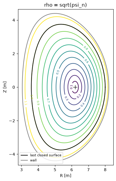
The field
Section titled “The field”magnetic_field(R, Z) returns (B_R, B_Z, B_phi) from the flux gradient, B_R = -(1/R) dpsi/dZ, B_Z = (1/R) dpsi/dR, and B_phi = F / R. The toroidal field falls off as 1/R, the poloidal field vanishes on the axis. magnetic_field_cartesian gives the same field at Cartesian points, which is how the deposition finds the pitch of each fast ion.
r_mid = np.linspace(boundary[:, 0].min(), boundary[:, 0].max(), 200)b_r, b_z, b_phi = (    np.asarray(b) for b in equilibrium.magnetic_field(r_mid, np.zeros_like(r_mid)))np.testing.assert_allclose(b_phi, B0 * R0 / r_mid, rtol=1e-12)assert abs(np.interp(R0, r_mid, b_z)) < 1e-3  # no poloidal field on the axis
fig, ax = plt.subplots(figsize=(6, 3.5), layout="constrained")ax.plot(r_mid, b_phi, label="B_phi")ax.plot(r_mid, b_z, label="B_Z")ax.axvline(R0, color="0.7", linestyle=":")ax.set_xlabel("R [m] on the midplane")ax.set_ylabel("B [T]")ax.legend()plt.show()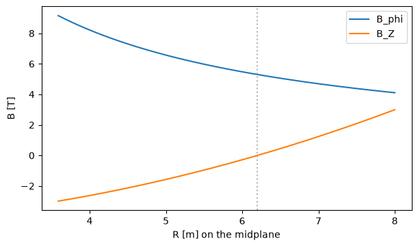
Flux shells
Section titled “Flux shells”flux_surfaces(rho_edges) cuts the plasma into shells between the given radii and returns their volumes, poloidal areas and inverse aspect ratios (R_max - R_min) / (R_max + R_min). The volumes are sums over a fine grid of cells, so their total must equal the volume of revolution of the boundary, 2 pi R_c A by Pappus’s theorem, with A the boundary’s area and R_c its centroid.
surfaces = equilibrium.flux_surfaces(np.linspace(0.0, 1.0, 21))
x, y = boundary[:, 0], boundary[:, 1]cross = x * np.roll(y, -1) - np.roll(x, -1) * yarea = 0.5 * cross.sum()centroid = ((x + np.roll(x, -1)) * cross).sum() / (6 * area)pappus = 2 * np.pi * centroid * abs(area)print(    f"shell volumes sum to {surfaces.volume.sum():.1f} m^3, Pappus gives {pappus:.1f} m^3")assert abs(surfaces.volume.sum() / pappus - 1) < 1e-3assert abs(surfaces.area.sum() / abs(area) - 1) < 1e-3
fig, (ax0, ax1) = plt.subplots(1, 2, figsize=(9, 3.2), layout="constrained")ax0.bar(surfaces.rho, surfaces.volume, width=np.diff(surfaces.rho_edges), edgecolor="k")ax0.set_xlabel("rho")ax0.set_ylabel("shell volume [m^3]")ax1.plot(surfaces.rho, surfaces.inverse_aspect_ratio, "o-")ax1.set_xlabel("rho")ax1.set_ylabel("inverse aspect ratio")plt.show()
shell volumes sum to 928.3 m^3, Pappus gives 928.3 m^3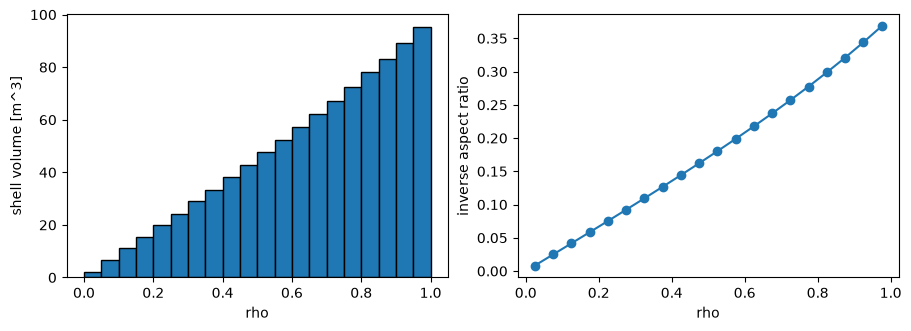
The outer shells hold most of the volume, which is why a beam that deposits near the edge needs a lot of power to change the central profiles. The inverse aspect ratio sets the share of trapped electrons in the current drive.
G-EQDSK files
Section titled “G-EQDSK files”Equilibrium.from_geqdsk(path) reads the equilibria that EFIT, CHEASE and other codes write, with the limiter as the wall; to_geqdsk writes one. The file is taken as it is: codes differ in the sign conventions of psi and the field (COCOS), so check the direction of B_phi and of the current for a file from another code. A round trip keeps the flux and the wall:
with tempfile.TemporaryDirectory() as directory:    path = Path(directory) / "solovev.geqdsk"    equilibrium.to_geqdsk(path)    reread = foc.Equilibrium.from_geqdsk(path)
difference = np.abs(np.asarray(reread.psi(r, z)) - np.asarray(equilibrium.psi(r, z)))[    inside].max()print(    f"round-trip flux difference: {difference / equilibrium.psi_boundary:.1e} of psi_boundary")assert difference < 1e-6 * equilibrium.psi_boundaryassert reread.wall is not None
round-trip flux difference: 9.6e-10 of psi_boundaryTry a smaller aspect ratio, Equilibrium.solovev(3.0, 1.0, 1.8, 2.0): the shells’ inverse aspect ratio, and with it the trapped-electron correction of the current, grows.