An injector from source to plasma: RF power and neutralizer gas against current drive.

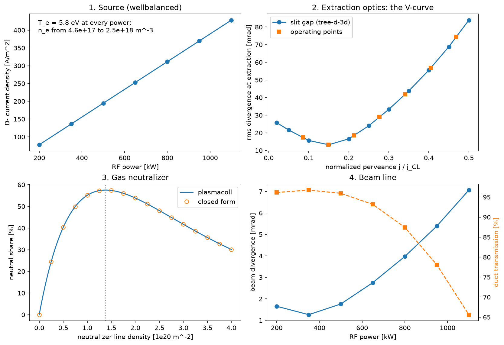
A negative-ion neutral-beam injector of ITER’s size, one stage per max-models code. The deuterium RF source is a wellbalanced global model: more RF power gives a denser plasma at the same electron temperature, and the extracted D- current density is taken as 30 % of the positive-ion Bohm flux to the plasma grid, from 78 A/m^2 at 200 kW to 430 A/m^2 at 1.1 MW. Against the Child-Langmuir limit of a 9 kV first gap of 6 mm, 914 A/m^2, that is a normalized perveance from 0.09 to 0.47, and over 0.2 m^2 of apertures a D- current from 16 to 86 A. The beamlet optics come from tree-d-3d: a slit extraction gap, solved with boundary-integral electrodes and meshless space charge, gives the classic V-curve of the divergence against the perveance, smallest near 0.15, and the acceleration to 1 MeV shrinks the angles by sqrt(9 kV / 1 MV), to 1.3-7 mrad. A fixed 70 % of the extracted ions survive the accelerator. The gas neutralizer is plasmacoll’s charge-state solution, whose neutral share peaks at 57.5 % near 1.4e20 m^-2 (and agrees with the closed form to 1e-14), and a 23 m duct of 0.5 m passes a share of the Gaussian beam that falls with its divergence. The neutral beam enters freeofcharge’s ITER-like plasma at a central density of 5e19 m^-3.

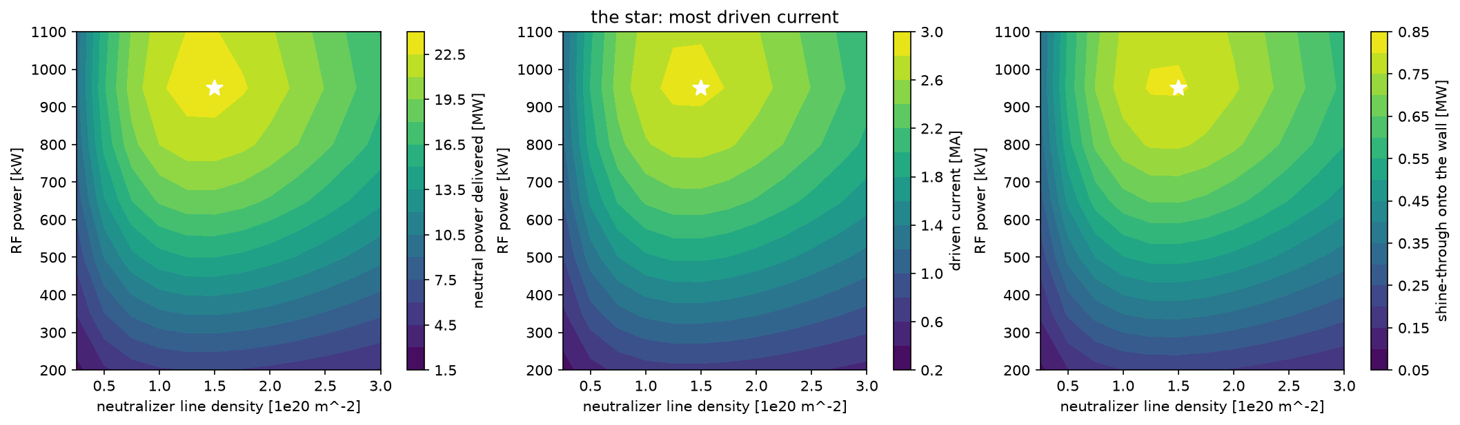
The two knobs pull against each other: more RF power gives more current but, past the optimum perveance, a more divergent beam, more of which the duct scrapes (65 % passes at 1.1 MW); more gas neutralizes more of the beam up to the maximum and then re-ionizes it. The scan maps the neutral power delivered, the driven current and the power shone through onto the inboard wall over the two: the most current, 2.9 MA from 23 MW, comes at 950 kW and a line density of 1.5e20 m^-2, next to the neutralizer’s optimum.

What is modelled, and what is not:

• Modelled: the source plasma’s particle and power balance (illustrative D2 rates, not data); space-charge-limited slit optics with a fixed emitter between 50-degree plasma-electrode wings; the charge states in a uniform gas cell (round-number cross sections of plausible size, not data); duct transmission of a Gaussian beam; the attenuation, slowing down and current drive in the plasma.
• Not modelled: negative-ion surface production on caesiated walls (the 30 % share is an input), co-extracted electrons, the plasma meniscus (whose curvature makes the real V-curve), round apertures and beamlet groups, stripping and optics in the accelerator (a fixed transmission and an adiabatic shrink of the angles), the residual-ion dump, re-ionization in the duct, and beam halos.

Python source

"""An injector from source to plasma: RF power and neutralizer gas against current drive.

A negative-ion neutral-beam injector of ITER's size, one stage per max-models code. The
deuterium RF source is a wellbalanced global model: more RF power gives a denser plasma
at the same electron temperature, and the extracted D- current density is taken as 30 %
of the positive-ion Bohm flux to the plasma grid, from 78 A/m^2 at 200 kW to 430 A/m^2
at 1.1 MW. Against the Child-Langmuir limit of a 9 kV first gap of 6 mm, 914 A/m^2,
that is a normalized perveance from 0.09 to 0.47, and over 0.2 m^2 of apertures a D-
current from 16 to 86 A. The beamlet optics come from tree-d-3d: a slit extraction gap,
solved with boundary-integral electrodes and meshless space charge, gives the classic
V-curve of the divergence against the perveance, smallest near 0.15, and the
acceleration to 1 MeV shrinks the angles by ``sqrt(9 kV / 1 MV)``, to 1.3-7 mrad. A
fixed 70 % of the extracted ions survive the accelerator. The gas neutralizer is
plasmacoll's charge-state solution, whose neutral share peaks at 57.5 % near
1.4e20 m^-2 (and agrees with the closed form to 1e-14), and a 23 m duct of 0.5 m passes
a share of the Gaussian beam that falls with its divergence. The neutral beam enters
freeofcharge's ITER-like plasma at a central density of 5e19 m^-3.

The two knobs pull against each other: more RF power gives more current but, past the
optimum perveance, a more divergent beam, more of which the duct scrapes (65 % passes at
1.1 MW); more gas neutralizes more of the beam up to the maximum and then re-ionizes it.
The scan maps the neutral power delivered, the driven current and the power shone
through onto the inboard wall over the two: the most current, 2.9 MA from 23 MW, comes
at 950 kW and a line density of 1.5e20 m^-2, next to the neutralizer's optimum.

What is modelled, and what is not:

- Modelled: the source plasma's particle and power balance (illustrative D2 rates, not
  data); space-charge-limited slit optics with a fixed emitter between 50-degree
  plasma-electrode wings; the charge states in a uniform gas cell (round-number cross
  sections of plausible size, not data); duct transmission of a Gaussian beam; the
  attenuation, slowing down and current drive in the plasma.
- Not modelled: negative-ion surface production on caesiated walls (the 30 % share is an
  input), co-extracted electrons, the plasma meniscus (whose curvature makes the real
  V-curve), round apertures and beamlet groups, stripping and optics in the accelerator
  (a fixed transmission and an adiabatic shrink of the angles), the residual-ion dump,
  re-ionization in the duct, and beam halos.
"""

import matplotlib.pyplot as plt
import numpy as np

import freeofcharge as foc
from freeofcharge import chain

RF_POWER = np.linspace(200e3, 1100e3, 7)  # W
LINE_DENSITY = np.linspace(0.25e20, 3.0e20, 12)  # m^-2
PERVEANCE = np.array([0.02, 0.05, 0.1, 0.15, 0.2, 0.25, 0.3, 0.35, 0.4, 0.45, 0.5])

EXTRACTION_VOLTAGE, GAP = 9.0e3, 6.0e-3  # V, m: the first (extraction) gap
APERTURE_AREA = 0.2  # m^2: 1280 apertures of 14 mm
BEAM_ENERGY = 1.0e6  # eV
ACCELERATOR_TRANSMISSION = 0.7  # share of the extracted ions that leave the accelerator
SOURCE_WIDTH, DUCT_LENGTH, DUCT_HALF_APERTURE = 0.1, 23.0, 0.25  # m

# 1. source: the current density against the RF power
sources = [chain.deuterium_source(p) for p in RF_POWER]
current_density = np.array([s.current_density for s in sources])
j_cl = chain.child_langmuir(EXTRACTION_VOLTAGE, GAP)
perveance = current_density / j_cl
current = current_density * APERTURE_AREA  # A of D-
# the slit optics are a converged fixed point only up to 0.5 (beyond, the beam reaches
# the extraction electrode and the iteration wanders): keep the scan inside it
assert perveance.max() <= PERVEANCE.max(), "RF power beyond the optics scan"

# 2. optics: the divergence against the perveance, then after the acceleration
curve, extracted = chain.slit_divergence(PERVEANCE)
assert np.all(extracted == 1.0), "the extraction electrode intercepts the beam"
shrink = np.sqrt(EXTRACTION_VOLTAGE / BEAM_ENERGY)
divergence = np.interp(perveance, PERVEANCE, curve) * shrink  # rad
transmission = np.array(
    [
        chain.duct_transmission(SOURCE_WIDTH, theta, DUCT_LENGTH, DUCT_HALF_APERTURE)
        for theta in divergence
    ]
)

# 3. neutralizer: the neutral share against the gas line density
pi_fine = np.linspace(0.0, 4.0e20, 401)
neutral_fine = chain.neutral_fraction(pi_fine)
neutral = chain.neutral_fraction(LINE_DENSITY)
best_pi = pi_fine[np.argmax(neutral_fine)]
print(
    f"neutralizer: at most {100 * neutral_fine.max():.1f} % neutral at "
    f"{best_pi:.2e} m^-2; closed form within "
    f"{np.abs(neutral_fine - chain.neutral_fraction_closed_form(pi_fine)).max():.0e}"
)

# 4. tokamak: shine-through and current per watt for each beam divergence
equilibrium = foc.Equilibrium.solovev(6.2, 1.8, 1.7, 5.3, wall_psi_n=1.3)
origin, direction = foc.tangential_injection(5.3, 12.0)
plasma = foc.Plasma.parabolic(5e19, 2.0e4, ions={"D": (2, 1, 0.96), "He": (4, 2, 0.02)})
rho_edges = np.linspace(0.0, 1.0, 21)
surfaces = equilibrium.flux_surfaces(rho_edges)
shine_fraction, current_per_watt = [], []
for theta in divergence:
    width = np.hypot(SOURCE_WIDTH, DUCT_LENGTH * theta)
    beam = foc.NeutralBeam.gaussian(
        origin, direction, BEAM_ENERGY, 1.0, width=width, divergence=theta,
        markers=1000, seed=1,
    )  # fmt: skip
    deposition = foc.deposit(
        beam, equilibrium, plasma, step=0.03, births_per_marker=2,
        rho_edges=rho_edges, seed=2,
    )  # fmt: skip
    steady = foc.slow_down(deposition, plasma, surfaces)
    shine_fraction.append(deposition.shine_through_fraction)
    current_per_watt.append(steady.driven_current / deposition.injected_power)
shine_fraction = np.array(shine_fraction)
current_per_watt = np.array(current_per_watt)

# the scan: neutral power into the torus, driven current, shine-through power
accelerated = current * BEAM_ENERGY * ACCELERATOR_TRANSMISSION  # W
delivered = (accelerated * transmission)[:, None] * neutral[None, :]
driven = delivered * current_per_watt[:, None]
shone = delivered * shine_fraction[:, None]
i, k = np.unravel_index(np.argmax(driven), driven.shape)
for s, p, theta, t in zip(sources, perveance, divergence, transmission, strict=True):
    print(
        f"{s.rf_power / 1e3:5.0f} kW: n_e {s.electron_density:.2e} m^-3, "
        f"j {s.current_density:4.0f} A/m^2, perveance {p:.2f}, "
        f"divergence {1e3 * theta:.1f} mrad, duct {100 * t:.0f} %"
    )
print(
    f"most current: {driven[i, k] / 1e6:.2f} MA from {delivered[i, k] / 1e6:.1f} MW "
    f"at {RF_POWER[i] / 1e3:.0f} kW and {LINE_DENSITY[k]:.2e} m^-2; "
    f"shine-through {100 * shine_fraction[i]:.1f} %"
)

fig, axes = plt.subplots(2, 2, figsize=(11, 7.5), layout="constrained")
ax = axes[0, 0]
ax.plot(RF_POWER / 1e3, current_density, "o-")
ax.set_xlabel("RF power [kW]")
ax.set_ylabel("D- current density [A/m^2]")
ax.set_title("1. Source (wellbalanced)")
ax.text(
    0.04,
    0.96,
    f"T_e = {sources[0].electron_temperature:.1f} eV at every power;\n"
    f"n_e from {sources[0].electron_density:.1e} to "
    f"{sources[-1].electron_density:.1e} m^-3",
    transform=ax.transAxes,
    va="top",
)
ax = axes[0, 1]
ax.plot(PERVEANCE, 1e3 * curve, "o-", label="slit gap (tree-d-3d)")
ax.plot(perveance, 1e3 * divergence / shrink, "s", color="C1", label="operating points")
ax.set_xlabel("normalized perveance j / j_CL")
ax.set_ylabel("rms divergence at extraction [mrad]")
ax.set_title("2. Extraction optics: the V-curve")
ax.legend()
ax = axes[1, 0]
ax.plot(pi_fine / 1e20, 100 * neutral_fine, label="plasmacoll")
ax.plot(
    pi_fine[::25] / 1e20,
    100 * chain.neutral_fraction_closed_form(pi_fine[::25]),
    "o",
    mfc="none",
    label="closed form",
)
ax.axvline(best_pi / 1e20, color="0.6", ls=":")
ax.set_xlabel("neutralizer line density [1e20 m^-2]")
ax.set_ylabel("neutral share [%]")
ax.set_title("3. Gas neutralizer")
ax.legend()
ax = axes[1, 1]
ax.plot(RF_POWER / 1e3, 1e3 * divergence, "o-", label="divergence after acceleration")
ax.set_xlabel("RF power [kW]")
ax.set_ylabel("beam divergence [mrad]")
ax.set_title("4. Beam line")
twin = ax.twinx()
twin.plot(RF_POWER / 1e3, 100 * transmission, "s--", color="C1")
twin.set_ylabel("duct transmission [%]", color="C1")

fig, axes = plt.subplots(1, 3, figsize=(14, 4), layout="constrained")
for ax, values, label, scale in (
    (axes[0], delivered, "neutral power delivered [MW]", 1e-6),
    (axes[1], driven, "driven current [MA]", 1e-6),
    (axes[2], shone, "shine-through onto the wall [MW]", 1e-6),
):
    mesh = ax.contourf(LINE_DENSITY / 1e20, RF_POWER / 1e3, values * scale, levels=14)
    fig.colorbar(mesh, ax=ax, label=label)
    ax.plot(LINE_DENSITY[k] / 1e20, RF_POWER[i] / 1e3, "w*", ms=12)
    ax.set_xlabel("neutralizer line density [1e20 m^-2]")
    ax.set_ylabel("RF power [kW]")
axes[1].set_title("the star: most driven current")

Plots