Designing the injection

Download notebook View on GitHubRun when the site was built.

Scan the beam energy and the tangency radius of an injector and weigh the shine-through onto the wall against the current the beam drives. This is the loop freeofcharge is built for: fast enough to sit inside an optimisation of the injector, at the end of the max-models chain from the ion source to the plasma.

Each configuration below deposits a 16.5 MW deuterium beam in an ITER-sized Solov’ev equilibrium and slows down its fast ions. The figure of merit for the current is the current-drive efficiency eta = R_0 n_e20 I / P [10^20 A/(W m^2)], with n_e20 the central density in 10^20 m^-3.

import matplotlib.pyplot as plt
import numpy as np

import freeofcharge as foc

R0 = 6.2
equilibrium = foc.Equilibrium.solovev(R0, 1.8, 1.7, 5.3, wall_psi_n=1.3)
ne0, power = 5e19, 16.5e6
plasma = foc.Plasma.parabolic(ne0, 1.5e4, ions={"D": (2, 1, 0.96), "He": (4, 2, 0.02)})
rho_edges = np.linspace(0.0, 1.0, 21)
surfaces = equilibrium.flux_surfaces(rho_edges)

energies = np.array([0.5e6, 0.75e6, 1.0e6, 1.5e6])
tangencies = np.array([4.5, 5.3, 6.0])
shine = np.zeros((len(tangencies), len(energies)))
current = np.zeros_like(shine)
for i, tangency in enumerate(tangencies):
    origin, direction = foc.tangential_injection(tangency, 12.0)
    for j, energy in enumerate(energies):
        beam = foc.NeutralBeam.gaussian(
            origin,
            direction,
            energy,
            power,
            width=0.3,
            divergence=0.005,
            markers=500,
            seed=1,
        )
        deposition = foc.deposit(
            beam,
            equilibrium,
            plasma,
            step=0.03,
            births_per_marker=2,
            rho_edges=rho_edges,
            seed=2,
        )
        shine[i, j] = deposition.shine_through_fraction
        current[i, j] = foc.slow_down(deposition, plasma, surfaces).driven_current
efficiency = R0 * (ne0 / 1e20) * current / power
print("shine-through [%]:\n", (100 * shine).round(2))
print("driven current [MA]:\n", (current / 1e6).round(2))

shine-through [%]:
 [[ 0.27  1.19  2.77  7.09]
 [ 0.36  1.48  3.3   8.05]
 [ 0.77  2.58  5.15 11.14]]
driven current [MA]:
 [[1.29 1.4  1.42 1.35]
 [1.44 1.56 1.58 1.51]
 [1.5  1.58 1.57 1.45]]

A faster beam reaches deeper and shines through more; a beam aimed further out has a shorter path through the plasma and shines through more as well. The current has a maximum in energy: it grows as the fast ions get faster, and falls again at the highest energy, where several percent of the power shine through. In this scan the beam tangent near the magnetic axis (5.3 m) drives more current than the one aimed inboard (4.5 m) at every energy.

assert np.all(np.diff(shine, axis=1) > 0)  # more energy: more shine-through
assert np.all(np.diff(shine, axis=0) > 0)  # aimed further out: more shine-through
assert np.all(current[1] > current[0])  # tangent near the axis beats inboard aiming

fig, (ax0, ax1) = plt.subplots(1, 2, figsize=(10, 3.8), layout="constrained")
for i, tangency in enumerate(tangencies):
    ax0.semilogy(energies / 1e6, 100 * shine[i], "o-", label=f"R_tan = {tangency} m")
    ax1.plot(energies / 1e6, efficiency[i], "o-", label=f"R_tan = {tangency} m")
ax0.set_xlabel("beam energy [MeV]")
ax0.set_ylabel("shine-through [%]")
ax1.set_xlabel("beam energy [MeV]")
ax1.set_ylabel("eta [10^20 A / (W m^2)]")
for ax in (ax0, ax1):
    ax.legend(fontsize=8)
plt.show()

best = np.unravel_index(
    np.argmax(np.where(shine < 0.05, efficiency, -np.inf)), shine.shape
)
print(
    f"best with under 5 % shine-through: {energies[best[1]] / 1e6:.2f} MeV, tangent to "
    f"R = {tangencies[best[0]]} m, eta = {efficiency[best]:.3f}, shine-through {100 * shine[best]:.2f} %"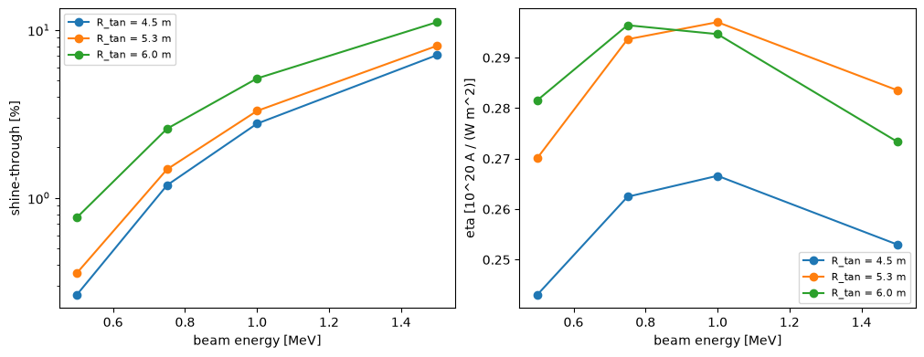
)

best with under 5 % shine-through: 1.00 MeV, tangent to R = 5.3 m, eta = 0.297, shine-through 3.30 %

The numbers show what the model computes, not ITER’s design: the Solov’ev shape is wider inboard than ITER’s, the profiles are parabolic, and the trapped-electron correction is a fit still to be checked. A real optimisation would also scan the density at which the beam is switched on, the vertical aiming (height), the divergence and the energy components, and add the constraint from the wall’s heat load: deposition.wall_hits gives where the shine-through lands.

Try a lower density, ne0 = 3e19: the shine-through limit then rules out the higher energies.