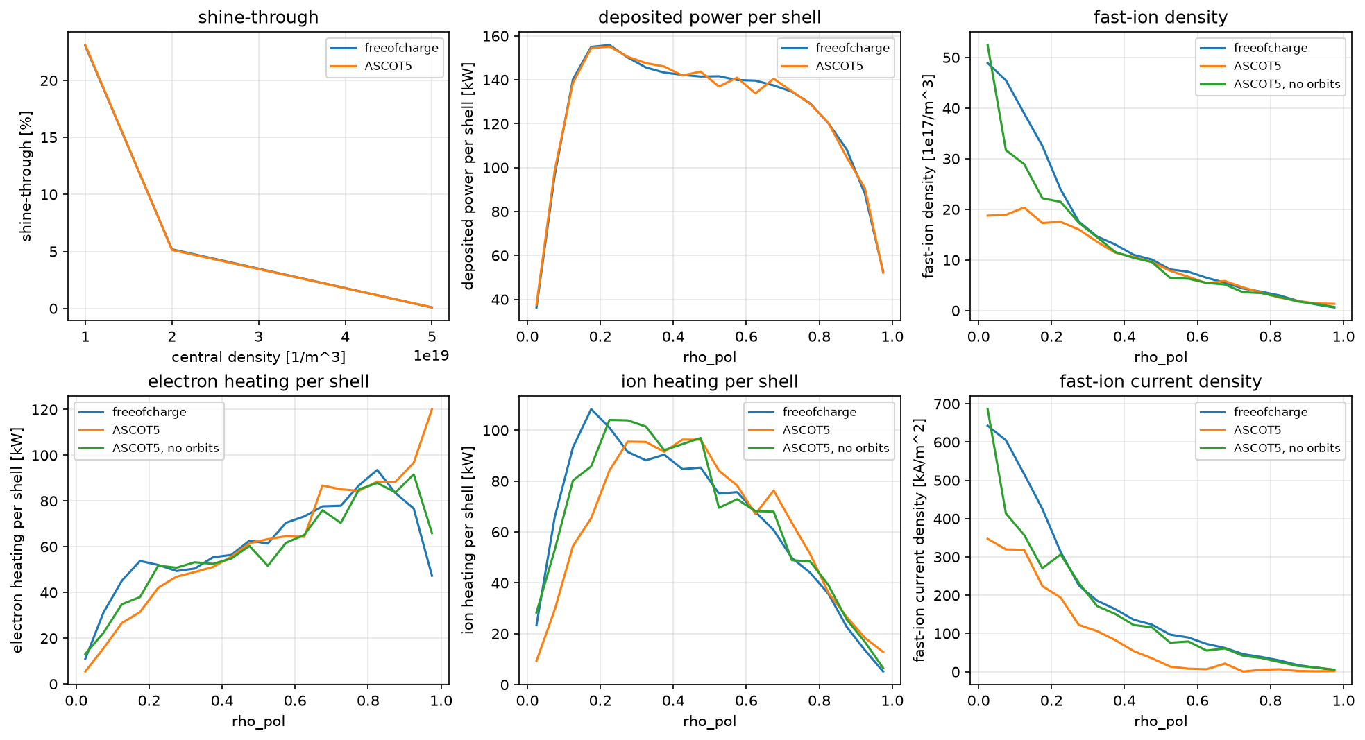
The ASCOT5 benchmark: deposition, shine-through, heating and current.

The case of freeofcharge.ascot5.benchmark_case, an ASDEX Upgrade-sized Solov’ev equilibrium with a 2.5 MW beam of 60 keV deuterium, computed by freeofcharge and compared with the ASCOT5 results stored in benchmarks/ascot5/ascot5_results.json. BBNBI5 gives the birth profile and the shine-through along the same lines (one beamlet per freeofcharge marker) with the same stopping cross sections (Suzuki’s fit), so the deposition agrees to within its Monte Carlo noise. ascot5_main slows the ions down twice, as guiding centres with Monte Carlo Coulomb collisions until 2 T_i: once following their orbits, and once without orbits, the markers staying where they were born as in freeofcharge’s local model. The heating agrees with both to 4%; the fast-ion current agrees with the run without orbits to 15% and is 2.7 times that of the run with orbits, since about 40% of the ions are born on trapped orbits (see the documentation page “ASCOT5 benchmark”).

Python source

"""The ASCOT5 benchmark: deposition, shine-through, heating and current.

The case of `freeofcharge.ascot5.benchmark_case`, an ASDEX Upgrade-sized
Solov'ev equilibrium with a 2.5 MW beam of 60 keV deuterium, computed by
freeofcharge and compared with the ASCOT5 results stored in
`benchmarks/ascot5/ascot5_results.json`. BBNBI5 gives the birth profile and
the shine-through along the same lines (one beamlet per freeofcharge marker)
with the same stopping cross sections (Suzuki's fit), so the deposition agrees
to within its Monte Carlo noise. ascot5_main slows the ions down twice, as
guiding centres with Monte Carlo Coulomb collisions until 2 T_i: once
following their orbits, and once without orbits, the markers staying where
they were born as in freeofcharge's local model. The heating agrees with both
to 4%; the fast-ion current agrees with the run without orbits to 15% and is
2.7 times that of the run with orbits, since about 40% of the ions are born
on trapped orbits (see the documentation page "ASCOT5 benchmark").
"""

from pathlib import Path

import numpy as np
import plasma_plots
import xarray as xr

from freeofcharge import ascot5

reference = ascot5.load_results(
    Path(__file__).resolve().parents[1]
    / "benchmarks"
    / "ascot5"
    / "ascot5_results.json"
)
local = ascot5.without_orbits(reference)
case = ascot5.benchmark_case(markers=reference["parameters"]["markers"])
ours = ascot5.run_freeofcharge(case)
print(ascot5.format_comparison(ascot5.compare(ours, reference)))
print()
print(ascot5.format_comparison(ascot5.compare(ours, local), "ASCOT5 local"))

rho_edges = np.asarray(ours["rho_edges"])
rho = 0.5 * (rho_edges[1:] + rho_edges[:-1])
runs = {"freeofcharge": ours, "ASCOT5": reference, "ASCOT5, no orbits": local}


def profile(name: str, scale: float, long_name: str, units: str, codes) -> xr.DataArray:
    """Return a profile of several runs, with a ``code`` axis."""
    return xr.DataArray(
        np.stack([np.asarray(runs[code][name]) for code in codes]) * scale,
        coords={"code": codes, "rho": ("rho", rho, {"long_name": "rho_pol"})},
        dims=("code", "rho"),
        attrs={"long_name": long_name, "units": units},
    )


deposition_codes = ["freeofcharge", "ASCOT5"]
codes = list(runs)
power = profile(
    "deposited_power", 1e-3, "deposited power per shell", "kW", deposition_codes
)
electrons = profile("electron_heating", 1e-3, "electron heating per shell", "kW", codes)
ions = profile("ion_heating", 1e-3, "ion heating per shell", "kW", codes)
density = profile("fast_ion_density", 1e-17, "fast-ion density", "1e17/m^3", codes)
current = profile(
    "fast_ion_current_density", 1e-3, "fast-ion current density", "kA/m^2", codes
)
shine = xr.DataArray(
    100
    * np.stack(
        [ours["scan_shine_through_fraction"], reference["scan_shine_through_fraction"]]
    ),
    coords={
        "code": deposition_codes,
        "ne0": (
            "ne0",
            np.asarray(ours["scan_ne0"]),
            {"long_name": "central density", "units": "1/m^3"},
        ),
    },
    dims=("code", "ne0"),
    attrs={"long_name": "shine-through", "units": "%"},
)

with plasma_plots.figure(2, 3, figsize=(13, 7)) as fig:
    shine.plasma.plot.profiles(x="ne0", over="code", ax=fig[0])
    power.plasma.plot.profiles(x="rho", over="code", ax=fig[1])
    density.plasma.plot.profiles(x="rho", over="code", ax=fig[2])
    electrons.plasma.plot.profiles(x="rho", over="code", ax=fig[3])
    ions.plasma.plot.profiles(x="rho", over="code", ax=fig[4])
    current.plasma.plot.profiles(x="rho", over="code", ax=fig[5])

Plots