Shapes and node masks

Download notebookView on GitHubRun when the site was built.

Test points against a shape, select the nodes it covers, and visualize the result.

The simgeometry.objects package includes Line in 1D; Circle, Rectangle, Triangle, Polygon, and apertures in 2D; and Sphere, Cuboid, Cylinder, Tube, SlantedTube, Cone, Torus, and apertures in 3D. The same contains(), contains_points(), and node_mask() pattern works across these shapes.

import numpy as np

from simgeometry.grid import Grid
from simgeometry.objects import Circle

grid = Grid(2, (0.0, 0.0), (1.0, 1.0), (41, 41))
circle = Circle(midpoint=(0.5, 0.5), radius=0.25)
mask = circle.node_mask(grid)
indices = circle.get_indices_in_object(grid)
print("mask shape:", mask.shape)
print("selected nodes:", len(indices))
assert indices == grid.indices_from_mask(mask)

mask shape: (41, 41)
selected nodes: 313

node_mask() is a host NumPy boolean array with the grid’s shape. Use get_indices_in_object() when you need integer node indices instead.

points = np.array([[0.5, 0.0, 0.8], [0.5, 0.0, 0.5]])
print("single point:", circle.contains((0.5, 0.5)))
print("point batch:", circle.contains_points(points))
assert circle.contains_points(points).tolist() == [True, False, False]

single point: True
point batch: [ True False False]

Batch points are component-major: the input shape is (ndim, N), with one point per column. To see where the mask lies on the grid, plot its selected nodes.

import matplotlib.pyplot as plt

nodes = grid.node_points()
fig, ax = plt.subplots(figsize=(5, 5))
ax.scatter(nodes[0], nodes[1], c=mask.ravel(), cmap="coolwarm", s=9)
ax.set(xlabel="x", ylabel="y", title="Grid nodes selected by Circle.node_mask")
ax.set_aspect("equal")
plt.show()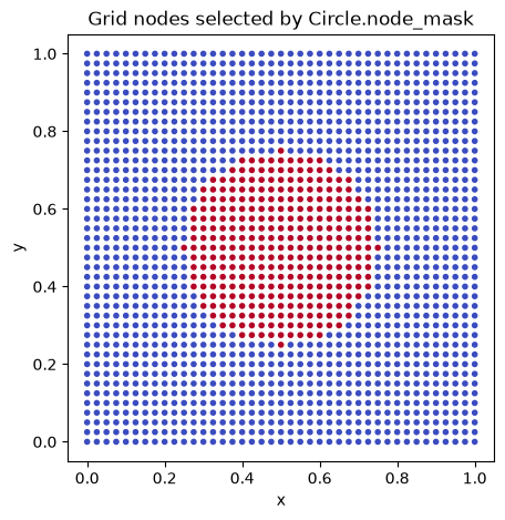

Inverted regions

Pass inverted=True to select the space outside a shape. The shape’s bounding box still describes its original geometry.

outside = Circle(midpoint=(0.5, 0.5), radius=0.25, inverted=True)
print("center selected:", outside.contains((0.5, 0.5)))
print("corner selected:", outside.contains((0.0, 0.0)))
assert np.array_equal(outside.node_mask(grid), ~mask)

center selected: False
corner selected: True

Rounded corners

Electrode fields are singular at sharp corners: the surface field on a rectangle’s corner grows without bound as the mesh is refined, while on a rounded one it converges. Rectangle(midpoint, side_lengths, fillet=r) rounds the four corners with radius r, up to half the shorter side, where it becomes a stadium. Cuboid(..., fillet=r) rounds the edges and corners of a box in the same way. The level set stays the exact signed distance, the outline is straight edges plus arcs, and crossings() stays analytic.

from simgeometry.objects import Rectangle

plate = Rectangle(midpoint=(0.5, 0.5), side_lengths=(0.8, 0.3), fillet=0.08)
stadium = Rectangle(midpoint=(0.5, 0.15), side_lengths=(0.8, 0.2), fillet=0.1)
(loop,) = plate.outlines(max_spacing=0.02)
print("outline vertices:", loop.shape[1])
print("distance from (1, 1):", plate.signed_distance((1.0, 1.0)))

fig, ax = plt.subplots(figsize=(5, 5))
for shape in (plate, stadium):
    inside = shape.node_mask(grid).ravel()
    ax.scatter(nodes[0][inside], nodes[1][inside], s=9)
    (outline,) = shape.outlines()
    ax.fill(*outline, fill=False)
ax.set(xlabel="x", ylabel="y", title="A rounded rectangle and a stadium")
ax.set_aspect("equal")
plt.show()

outline vertices: 106
distance from (1, 1): 0.38615448083226656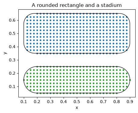

Solids in three dimensions

Besides Sphere and Cuboid, 3D geometry has solids of revolution along any axis: Cylinder(start, end, radius), Tube(start, end, inner_radius, outer_radius) for rings and drift tubes, Cone(start, end, start_radius, end_radius) for cones and frustums, and Torus(midpoint, major_radius, minor_radius, axis=...). Cylinder and Tube take an optional fillet that rounds their circular edges.

With simgeometry[interactive], show_3d(backend="pyvista") draws a collection with one colour per object, and plasma_plots.scene shows it as an interactive scene. Click Interactive 3-D view below the picture, then rotate it to look along the tilted cylinder and into the bore of the tube.

import plasma_plots
import pyvista as pv

from simgeometry import Cone, Cylinder, GeometryCollection, Torus, Tube

pv.OFF_SCREEN = True  # render without a window, e.g. on a docs server

solids = GeometryCollection(
    {
        "cylinder": Cylinder((-0.4, 0.4, -0.5), (0.4, -0.4, 0.5), 0.3),
        "tube": Tube((2, 0, -0.5), (2, 0, 0.5), 0.35, 0.65, fillet=0.1),
        "cone": Cone((0, 2, -0.5), (0, 2, 0.6), 0.6, 0.0),
        "torus": Torus((2, 2, 0), 0.55, 0.18, axis=(1, 0, 1)),
    }
)
assert solids["tube"].contains((2.5, 0, 0))
assert not solids["tube"].contains((2, 0, 0))  # the bore is empty
plotter = solids.show_3d(
    backend="pyvista", display=False, resolution=56, show_bounds=False
)
plasma_plots.scene(
    plotter,
    alt="A tilted cylinder, a tube with rounded edges, a cone and a tilted torus, "
    "one colour each",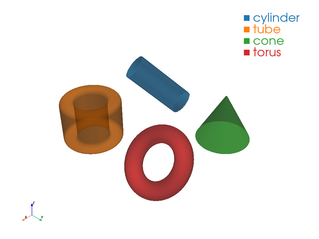
)

Interactive 3-D view (2.1 MB)Open in a new tab

A tube with a slanted end

SlantedTube(start, end, inner_radius, outer_radius, cut_normal) is a tube whose end at end is cut by the plane through end with the outward normal cut_normal, like the mouth of a caesium oven nozzle cut at 45°; inner_radius=0 gives a solid rod. Its level set is a bound on the distance (exact on the faces), and crossings with it are analytic, so particles bouncing inside a thin duct find every wall. Below, steps from inside the bore to random points in all directions: the ones that leave through the open mouth have no crossing, the others stop on the wall.

from simgeometry import SlantedTube
from simgeometry.crossings import crossings

c = np.cos(np.pi / 4)
nozzle = SlantedTube((0, 0, 0), (0, 0, 1.0), 0.15, 0.2, (0, -c, c))
print(f"cut angle {nozzle.cut_angle:.0f} deg, volume {nozzle.volume():.4f}")
rng = np.random.default_rng(0)
count = 400
start = np.zeros((3, count))
start[2] = 0.8  # on the axis, inside the bore
direction = rng.normal(size=(3, count))
direction /= np.linalg.norm(direction, axis=0)
hits = crossings(nozzle, start, start + 2.0 * direction)
print("steps stopped by the wall:", int(hits.hit.sum()), "of", count)
plotter = nozzle.show_3d(
    backend="pyvista",
    display=False,
    resolution=64,
    opacity=0.3,
    show_bounds=False,
    points={
        "crossings": {
            "points": hits.point[:, hits.hit],
            "vectors": hits.normal[:, hits.hit],
        }
    },
)
plasma_plots.scene(
    plotter, alt="A tube cut at 45 degrees, with the crossings of steps from its bore"
)

cut angle 45 deg, volume 0.0550
steps stopped by the wall: 348 of 400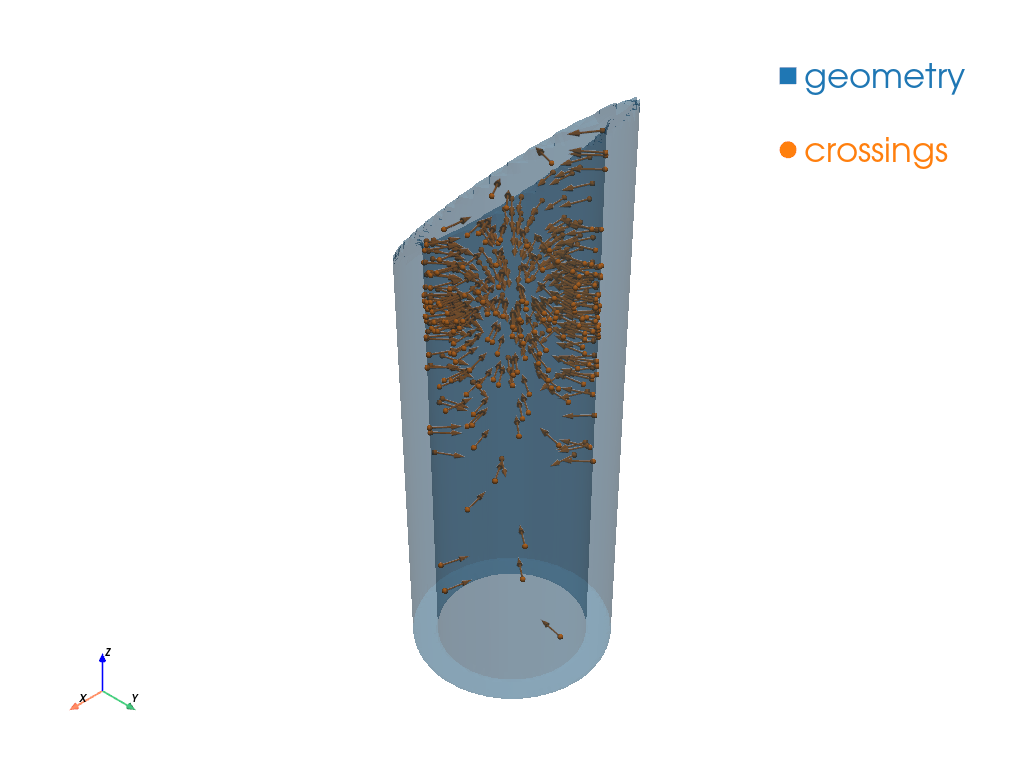

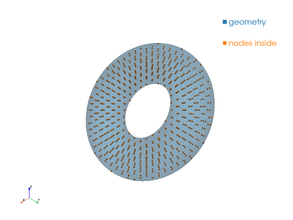
Interactive 3-D view (1.7 MB)Open in a new tab

node_mask() works the same way on a 3D grid. show_3d(points=...) draws the nodes inside a tilted torus as a labelled point set over its translucent surface, in simgeometry’s (3, n) layout as node_points() returns them; rotate the view to see that they fill the tube of the torus and leave its hole empty.

grid3 = Grid(3, (-1.0, -1.0, -1.0), (1.0, 1.0, 1.0), (21, 21, 21))
torus = Torus((0, 0, 0), 0.6, 0.25, axis=(1, 0, 1))
mask3 = torus.node_mask(grid3)
print("selected nodes:", mask3.sum(), "of", mask3.size)
plotter = torus.show_3d(
    backend="pyvista",
    display=False,
    resolution=48,
    opacity=0.3,
    show_bounds=False,
    points={"nodes inside": grid3.node_points()[:, mask3.ravel()]},
)
plasma_plots.scene(
    plotter, alt="The grid nodes inside a tilted torus, drawn inside its surface"
)

selected nodes: 758 of 9261

Interactive 3-D view (1.2 MB)Open in a new tab