Sampling, export and diagnostics

Download notebookView on GitHubRun when the site was built.

Sample interior and boundary points, export contours and surface meshes, and inspect geometric resolution before running a simulation. All meshes and quadrature results carry a sampling resolution; they should be refined for small features.

from pathlib import Path
from tempfile import TemporaryDirectory

import matplotlib.pyplot as plt
import numpy as np

from simgeometry import Circle, GeometryCollection, Grid, Sphere

sphere = Sphere((0, 0, 0), 1)
inside = sphere.sample_interior(1000, rng=7)
assert sphere.contains_points(inside).all()
np.testing.assert_array_equal(inside, sphere.sample_interior(1000, rng=7))
surface = sphere.sample_surface(600, rng=7, resolution=32)
print(
    "Largest radial mesh sampling error:",
    np.max(abs(np.linalg.norm(surface, axis=0) - 1)),
)
fig = plt.figure(figsize=(10, 4), layout="constrained")
for index, points, title in (
    (1, inside, "Uniform interior samples"),
    (2, surface, "Samples by mesh surface area"),
):
    ax = fig.add_subplot(1, 2, index, projection="3d")
    ax.scatter(*points, s=3, alpha=0.5)
    ax.set_box_aspect((1, 1, 1))
    ax.set_title(title)
plt.show()

Largest radial mesh sampling error: 0.0017257751355151951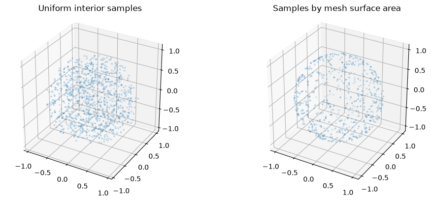

Interior sampling uses rejection sampling with a finite draw budget. Pass a seed or NumPy Generator for reproducibility, and explicit bounds for inverted/unbounded objects. Exhausting max_draws raises an error instead of returning too few points.

Surface sampling is uniform by segment length in 2D and triangle area in 3D, on the extracted mesh. Those points approximate the mathematical surface; they need not satisfy exact boundary membership.

A shape with a hole shows the two samplers best. On the left, interior samples of a torus; on the right, surface samples of the same torus, each over its translucent surface. show_3d(points=...) draws the (3, n) samples as labelled point sets, with a legend entry beside the objects. Click Interactive 3-D view and turn the scene: the interior points fill the tube and leave the hole empty, while the surface points lie on the faceted mesh.

import plasma_plots
import pyvista as pv

from simgeometry import Torus

pv.OFF_SCREEN = True  # render without a window, e.g. on a docs server

tori = GeometryCollection(
    {
        "left torus": Torus((0, 0, 0), 0.7, 0.3),
        "right torus": Torus((0, 2.4, 0), 0.7, 0.3),
    }
)
interior = tori["left torus"].sample_interior(1500, rng=7)
boundary = tori["right torus"].sample_surface(1000, rng=7, resolution=48)
assert tori["left torus"].contains_points(interior).all()
plotter = tori.show_3d(
    backend="pyvista",
    display=False,
    resolution=48,
    opacity=0.25,
    show_bounds=False,
    points={
        "interior samples": {"points": interior, "size": 5},
        "surface samples": {"points": boundary, "size": 5},
    },
)
plasma_plots.scene(
    plotter,
    alt="Interior samples filling a torus, and surface samples on a second torus",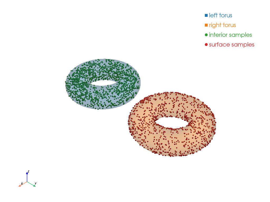
)

Interactive 3-D view (1.5 MB)Open in a new tab

Distance queries

Balls, boxes and simple polygons have exact closest-point and signed-distance queries. The sign is negative inside. Composite shapes, arbitrary functions and general affine images use the nearest point on a sampled boundary mesh. This is a distance approximation, and it can miss unresolved pieces.

ring = Circle((0, 0), 1.0) - Circle((0, 0), 0.4)
points = np.array([[0.0, 0.7, 1.3], [0.0, 0.0, 0.0]])
print("Approximate ring distances:", ring.signed_distance(points, resolution=128))
print("Closest ring points:", ring.closest_point(points, resolution=128))
np.testing.assert_allclose(
    ring.signed_distance(points, resolution=128), [0.4, -0.3, 0.3], atol=0.03
)

Approximate ring distances: [ 0.39984678 -0.29996249  0.30003751]
Closest ring points: [[-2.25410088e-01  9.99962487e-01  9.99962487e-01]
 [-3.30254053e-01  1.73472348e-18  1.73472348e-18]]

Portable mesh export

to_mesh() returns physical vertices, connectivity and grid spacing. NPZ preserves arrays; OBJ supports 2D segments and 3D triangles; STL supports 3D triangles. Sampling bounds can clip a surface, leaving it open. Export does not automatically cap it or certify a watertight solid.

mesh = sphere.to_mesh(resolution=32)
print("Vertices:", mesh.vertices.shape, "Triangles:", mesh.cells.shape)
print("Sampling spacing:", mesh.spacing)
with TemporaryDirectory() as directory:
    for suffix in ("npz", "obj", "stl"):
        path = mesh.save(Path(directory) / f"sphere.{suffix}")
        print(path.name, path.stat().st_size, "bytes")
    restored = np.load(Path(directory) / "sphere.npz")
    np.testing.assert_array_equal(restored["cells"], mesh.cells)
# To keep a mesh: sphere.export("sphere.stl", resolution=64)

Vertices: (3696, 3) Triangles: (7388, 3)
Sampling spacing: (0.07096774193548394, 0.07096774193548394, 0.07096774193548394)
sphere.npz 222446 bytes
sphere.obj 353700 bytes
sphere.stl 2262046 bytes

Diagnose overlaps and resolution

Diagnostics report overlapping solid nodes, objects with no solid node, multiple hits on an edge and hits very close to an endpoint. These are sampled observations, not proof that a geometry is resolved. A tiny object away from all grid edges may still escape detection.

grid = Grid(ndim=2, lower_bound=(-1, -1), upper_bound=(1, 1), num_gridpoints=(13, 13))
geometry = GeometryCollection(
    {
        "left": Circle((-0.15, 0), 0.4),
        "right": Circle((0.15, 0), 0.4),
        "small": Circle((0.74, 0.74), 0.01),
    }
)
report = geometry.diagnose(grid)
print(report)
assert report["overlap_nodes"]["left / right"] > 0
assert "small" in report["objects_without_solid_nodes"]
geometry.show(grid=grid, display=False)
plt.title("Overlapping objects and an unresolved small component")
plt.show()

{'overlap_nodes': {'left / right': 11}, 'objects_without_solid_nodes': ['small'], 'multiple_hit_edges': 0, 'short_distance_hits': 0, 'intersection_search_exact': True, 'scope': 'node and edge samples; does not certify feature resolution'}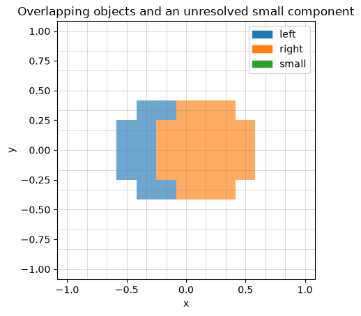

Repeat the diagnostics on a finer grid, then vary the sampling used for a function-defined shape. For finite-volume experiments, compare cell_fractions() estimates at several subcell resolutions before using them in a conservation calculation.