Parallel grids

Download notebookView on GitHubRun when the site was built.

Inspect the MPI decomposition of a structured grid. The first example runs on one process; the same constructor accepts an MPI communicator for parallel runs.

Decomposition metadata

Choose which axes may be split with domain_decomposition. On one process, the index bounds cover the full grid. num_ghost_points adds ghost nodes on both sides of each local axis.

from simgeometry.grid import Grid

grid = Grid(
    ndim=2,
    lower_bound=(0.0, 0.0),
    upper_bound=(1.0, 1.0),
    num_gridpoints=(18, 12),
    domain_decomposition=(True, False),
    num_ghost_points=1,
    periodic=(True, False),
)
print("rank:", grid.mpi_rank)
print("process grid:", grid.proc_sizes)
print("global index bounds:", grid.proc_index_bounds)
print("local shape with ghosts:", grid.num_gridpoints_local_with_ghosts)

rank: 0
process grid: [1, 1]
global index bounds: [(0, 18), (0, 12)]
local shape with ghosts: (20, 14)

For a multi-process run, install simgeometry[mpi], pass comm=MPI.COMM_WORLD, and launch the script with mpiexec -n 4 python script.py:

from mpi4py import MPI
from simgeometry.grid import Grid

grid = Grid(
    ndim=2,
    lower_bound=(0.0, 0.0),
    upper_bound=(1.0, 1.0),
    num_gridpoints=(18, 12),
    comm=MPI.COMM_WORLD,
    domain_decomposition=(True, True),
    num_ghost_points=1,
)
print(grid.mpi_rank, grid.proc_index_bounds, grid.num_gridpoints_local)

proc_index_bounds contains half-open global index ranges. neighbor_ranks gives lower and upper neighbors per axis, using MPI.PROC_NULL at nonperiodic walls. grid.domain_decomposition_class.layout(shape, halo=...) returns a matching mpiarray.Layout for field arrays.

Preview a decomposition

Without a communicator there is one process, so the grid above is never split. DomainDecomposition.preview(size, ...) builds the decomposition a size-rank run would use, without MPI: the same processes per axis, index ranges and subdomains, for every rank. It is for inspection and planning; nothing communicates, and it has no array layout. proc_sizes= fixes the processes per axis instead of size.

from simgeometry.domain_decomposition import DomainDecomposition

lower, upper, nodes = (0.0, 0.0, 0.0), (2.0, 1.0, 1.0), (33, 17, 17)
preview = DomainDecomposition.preview(8, decompose=[True, True, True])
print("process grid:", preview.proc_sizes)
for rank in range(preview.mpi_size):
    print(
        f"rank {rank}: coordinate {preview.get_proc_coord(rank)},",
        f"nodes {preview.get_index_bounds(nodes, rank)}",
    )
print(
    "owner of (1.5, 0.2, 0.9):",
    preview.owner_rank_for_position((1.5, 0.2, 0.9), lower, upper, nodes),
)

process grid: [2, 2, 2]
rank 0: coordinate (0, 0, 0), nodes [(0, 17), (0, 9), (0, 9)]
rank 1: coordinate (0, 0, 1), nodes [(0, 17), (0, 9), (9, 17)]
rank 2: coordinate (0, 1, 0), nodes [(0, 17), (9, 17), (0, 9)]
rank 3: coordinate (0, 1, 1), nodes [(0, 17), (9, 17), (9, 17)]
rank 4: coordinate (1, 0, 0), nodes [(17, 33), (0, 9), (0, 9)]
rank 5: coordinate (1, 0, 1), nodes [(17, 33), (0, 9), (9, 17)]
rank 6: coordinate (1, 1, 0), nodes [(17, 33), (9, 17), (0, 9)]
rank 7: coordinate (1, 1, 1), nodes [(17, 33), (9, 17), (9, 17)]
owner of (1.5, 0.2, 0.9): 5

subdomain_boxes(lower, upper, num_gridpoints) returns every rank’s (lower, upper) corners. show_3d draws them as translucent boxes, one colour per rank, with an optional shape inside (click Interactive 3-D view below the picture to rotate it). Rank 0 sits at the lower corner; ranks are numbered row-major, so the last axis changes fastest.

import plasma_plots
import pyvista as pv

from simgeometry import Sphere

pv.OFF_SCREEN = True  # render without a window, e.g. on a docs server

plotter = preview.show_3d(
    lower, upper, nodes, shape=Sphere((1.0, 0.5, 0.5), 0.35), display=False
)
plasma_plots.scene(
    plotter, alt="Eight subdomains, one colour per rank, around a sphere"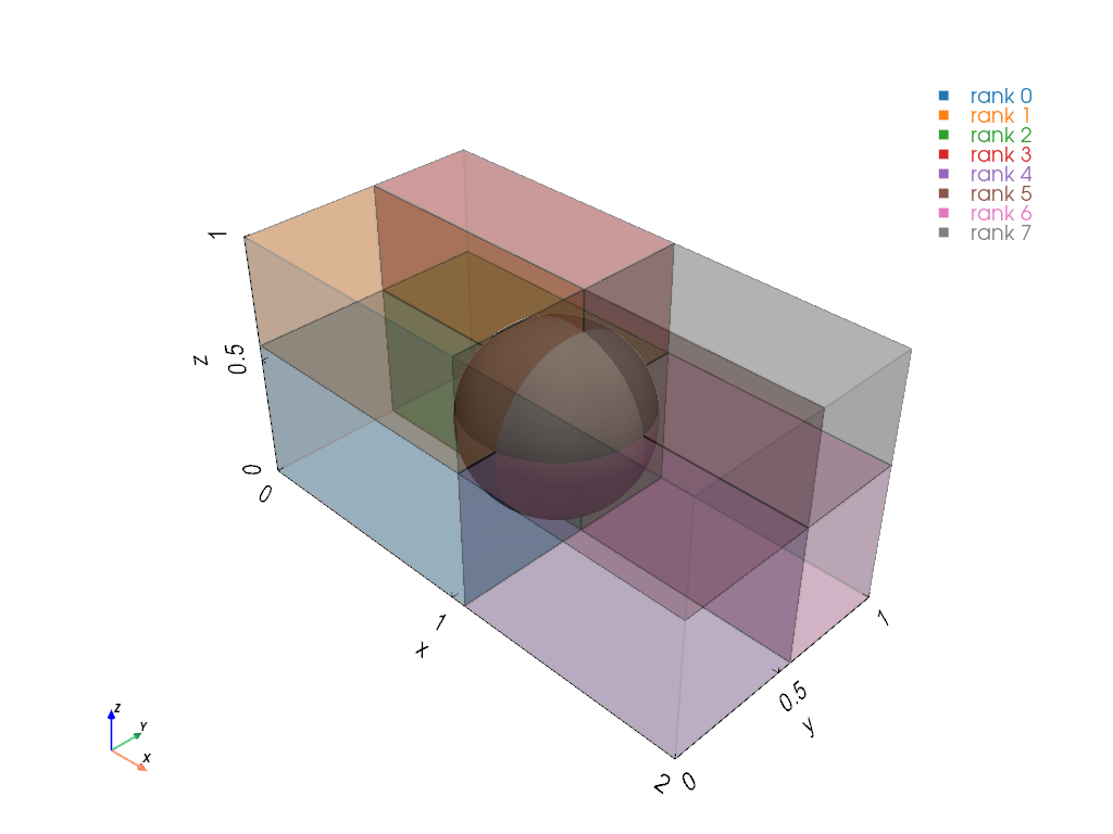
)

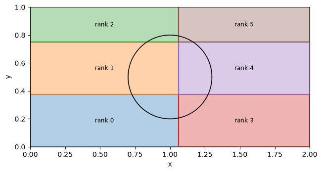
Interactive 3-D view (1.3 MB)Open in a new tab

A 2D decomposition has a Matplotlib view, show: one rectangle per rank, with a shape outlined on top. Six ranks on a 2D grid make a 2 × 3 process grid.

from simgeometry import Circle

DomainDecomposition.preview(6, ndim=2).show(
    (0.0, 0.0), (2.0, 1.0), (33, 17), shape=Circle((1.0, 0.5), 0.3)
);