Boundary outlines

Download notebookView on GitHubRun when the site was built.

Turn a 2D shape into closed loops of boundary vertices, at a resolution you choose. Boundary-element and panel solvers discretise electrodes and walls from these loops; they also give perimeters, areas and plot outlines.

shape.outlines(max_spacing=None) returns a list of (2, n) NumPy arrays, one per piece of the shape. Each loop is counter-clockwise and does not repeat its first vertex.

import matplotlib.pyplot as plt
import numpy as np

from simgeometry import Aperture2D, Circle, Polygon, Polyline, Rectangle

rectangle = Rectangle(midpoint=(0.0, 0.0), side_lengths=(2.0, 1.0))
(loop,) = rectangle.outlines()
print(loop)
assert loop.shape == (2, 4)

[[-1.   1.   1.  -1. ]
 [-0.5 -0.5  0.5  0.5]]

Without max_spacing, a polygon’s outline is its corners and a circle gets 100 vertices. A shape made of several pieces has one loop per piece: an Aperture2D has a lower and an upper plate. Aperture2D.slit() builds the common rectangular plates; axis=1 turns the beam along y. Inverting a shape does not change its outline.

slit = Aperture2D.slit(0.0, half_width=0.3, thickness=0.5, length=0.9)
shapes = {
    "rectangle": rectangle,
    "circle": Circle(midpoint=(0.0, 0.0), radius=0.6),
    "L-shaped polygon": Polygon(
        vertices=np.array([(0, 0), (2, 0), (2, 1), (1, 1), (1, 2), (0, 2)], dtype=float)
    ),
    "slit aperture": slit,
}

fig, axes = plt.subplots(1, 4, figsize=(12, 3), layout="constrained")
for ax, (name, shape) in zip(axes, shapes.items()):
    for loop in shape.outlines():
        closed = np.concatenate((loop, loop[:, :1]), axis=1)
        ax.plot(*closed, "-o", markersize=3)
    ax.set_title(f"{name}: {len(shape.outlines())} loop(s)")
    ax.set_aspect("equal")
axes[-1].set_xticks([-0.25, 0.25])
plt.show()

assert len(slit.outlines()) == 2
inverted = Circle(midpoint=(0.0, 0.0), radius=0.6, inverted=True)
np.testing.assert_array_equal(inverted.outlines()[0], shapes["circle"].outlines()[0])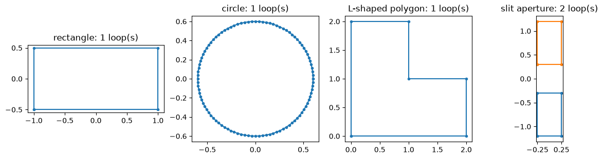

Choosing the spacing

With a number for max_spacing, every edge longer than it is split into equal pieces, so no two consecutive vertices are further apart. Polygon corners stay exact. On a circle every vertex lies on the circle, so the loop is an inscribed polygon whose perimeter and area converge as the spacing shrinks.

def perimeter(loop):
    closed = np.concatenate((loop, loop[:, :1]), axis=1)
    return np.hypot(*np.diff(closed, axis=1)).sum()


def area(loop):
    x, y = loop
    return 0.5 * np.sum(x * np.roll(y, -1) - np.roll(x, -1) * y)


circle = Circle(midpoint=(0.0, 0.0), radius=1.0)
spacings = [0.8, 0.4, 0.2, 0.1, 0.05, 0.025]
perimeter_error, area_error = [], []
for spacing in spacings:
    (loop,) = circle.outlines(max_spacing=spacing)
    closed = np.concatenate((loop, loop[:, :1]), axis=1)
    assert np.hypot(*np.diff(closed, axis=1)).max() <= spacing + 1e-12
    np.testing.assert_allclose(np.hypot(*loop), 1.0)
    perimeter_error.append(2 * np.pi - perimeter(loop))
    area_error.append(np.pi - area(loop))
    print(f"max_spacing {spacing:5.3f}: {loop.shape[1]:4d} vertices")

fig, ax = plt.subplots(figsize=(5, 3.5), layout="constrained")
ax.loglog(spacings, perimeter_error, "o-", label="perimeter error")
ax.loglog(spacings, area_error, "s-", label="area error")
ax.loglog(spacings, 0.2 * np.square(spacings), "k--", label="spacing²")
ax.set_xticks(spacings, [f"{spacing:g}" for spacing in spacings], minor=False)
ax.set_xticks([], minor=True)
ax.set_xlabel("max_spacing")
ax.set_ylabel("error of the inscribed polygon")
ax.legend()
plt.show()

(l_shape,) = shapes["L-shaped polygon"].outlines(max_spacing=0.25)
assert area(l_shape) == 3.0  # refining a polygon only adds points on its edges

max_spacing 0.800:    8 vertices
max_spacing 0.400:   16 vertices
max_spacing 0.200:   32 vertices
max_spacing 0.100:   63 vertices
max_spacing 0.050:  126 vertices
max_spacing 0.025:  252 vertices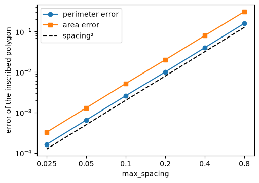

Both errors fall as the square of the spacing, the accuracy of a polygon inscribed in a smooth curve.

Graded spacing

max_spacing can also be a function: it takes (2, m) points and returns (m,) spacings. Vertices are then placed at about the local spacing, so you can resolve a corner or an aperture tip finely and keep the rest coarse. A boundary-element solver needs short panels where the field varies fastest, and a slit’s field varies fastest at its tip. With a function, the spacing holds approximately, not as a strict bound.

def tip_spacing(points):
    """0.02 at the slit tips (|y| = 0.3), growing with distance, at most 0.2."""
    distance = np.abs(points[1]) - 0.3
    return np.minimum(0.02 + 0.25 * distance, 0.2)


uniform = slit.outlines(max_spacing=0.02)
graded = slit.outlines(max_spacing=tip_spacing)
n_uniform = sum(loop.shape[1] for loop in uniform)
n_graded = sum(loop.shape[1] for loop in graded)
print("vertices, uniform 0.02:", n_uniform)
print("vertices, graded:      ", n_graded)

fig, (ax0, ax1) = plt.subplots(
    1, 2, figsize=(10, 3.5), layout="constrained", width_ratios=(1, 2)
)
for loop in graded:
    closed = np.concatenate((loop, loop[:, :1]), axis=1)
    ax0.plot(*closed, "-o", markersize=2)
ax0.set_aspect("equal")
ax0.set_xticks([-0.25, 0.25])
ax0.set_title("Graded vertices on the slit")

upper = graded[1]
closed = np.concatenate((upper, upper[:, :1]), axis=1)
midpoints = 0.5 * (closed[:, 1:] + closed[:, :-1])
edges = np.hypot(*np.diff(closed, axis=1))
order = np.argsort(midpoints[1])
ax1.plot(midpoints[1][order], edges[order], ".", label="edge length")
y = np.linspace(0.3, 1.2, 200)
ax1.plot(y, tip_spacing(np.stack((np.zeros_like(y), y))), "k-", label="requested")
ax1.set_xlabel("y (distance along the plate)")
ax1.set_ylabel("spacing")
ax1.legend()
plt.show()

assert edges[midpoints[1] < 0.35].max() < 0.03
assert n_graded < n_uniform / 2

vertices, uniform 0.02: 280
vertices, graded:       100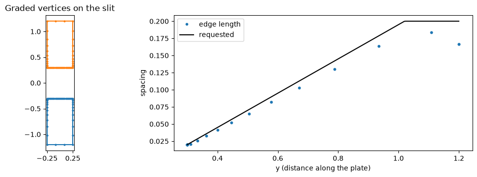

The graded outline matches the uniform one at the tip with about a third of the vertices. Edges come out at or a little below the requested spacing, because each edge of the shape is split into a whole number of pieces.

Transformed shapes

Shapes from translated(), rotated(), scaled() and transformed() have outlines too: the source’s loops, mapped by the transform. The spacing applies after the transform, both as a number and as a function of world coordinates.

bar = Rectangle(midpoint=(0.0, 0.0), side_lengths=(2.0, 0.4))
tilted = bar.rotated(30).scaled((1.0, 2.0)).translated((1.0, 0.5))
(loop,) = tilted.outlines(max_spacing=0.1)
closed = np.concatenate((loop, loop[:, :1]), axis=1)
assert np.hypot(*np.diff(closed, axis=1)).max() <= 0.1 + 1e-12
assert area(loop) > 0  # still counter-clockwise

(source,) = bar.outlines()
fig, ax = plt.subplots(figsize=(5, 3.5), layout="constrained")
ax.plot(*np.concatenate((source, source[:, :1]), axis=1), "k--", label="source")
ax.plot(*closed, "-o", markersize=2, label="rotated, scaled, translated")
ax.set_aspect("equal")
ax.legend()
plt.show()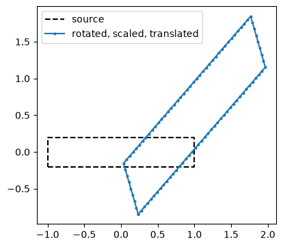

Holes and open curves

Boolean shapes (a | b, a & b, a - b, nested) have outlines through shapely (pip install 'simgeometry[clip]'). Every loop keeps the shape on its left: outer boundaries run counter-clockwise and holes clockwise. Each operand enters as the polygon of its own outline, so a circle stays an inscribed polygon.

A Polyline is an open curve of zero thickness, such as a thin plate or a wire. It encloses no area, so contains is always false and closed is False; its outline runs from its first vertex to its last.

plate = Rectangle(midpoint=(0.0, 0.0), side_lengths=(3.0, 2.0)) - Circle(
    (0.5, 0.0), 0.5
)
outer, hole = plate.outlines(max_spacing=0.1)
assert area(outer) > 0 > area(hole)  # counter-clockwise outside, clockwise hole
assert abs(area(outer) + area(hole) - (6.0 - np.pi * 0.25)) < 0.01

grid_wire = Polyline([(-1.2, -1.9), (0.0, -1.6), (1.2, -1.9)])
assert grid_wire.closed is False and not grid_wire.contains((0.0, -1.6))
(wire,) = grid_wire.outlines(max_spacing=0.1)
assert wire.shape[1] > 2  # refined, still open: no edge back to the start

Panels for boundary-element solvers

boundary_panels(max_spacing) turns the outline into straight panels with midpoints, lengths and unit normals. The normal is to the right of each panel’s direction; since loops keep the shape on their left, it points out of the geometry, into the hole for a hole. For an open curve it is the side to the right of the curve’s direction.

fig, ax = plt.subplots(figsize=(6, 4.5), layout="constrained")
for shape in (plate, grid_wire):
    panels = shape.boundary_panels(max_spacing=0.15)
    for piece in np.unique(panels.piece):
        own = panels.piece == piece
        ends = np.concatenate(
            (panels.start[:, own], panels.end[:, own][:, -1:]), axis=1
        )
        ax.plot(*ends, "k-", linewidth=1)
    ax.quiver(*panels.midpoint, *panels.normal, angles="xy", scale=30, width=0.003)
    print(
        f"{type(shape).__name__}: {len(panels)} panels, total length {panels.length.sum():.3f}"
    )
ax.set_aspect("equal")
ax.set_title(
    "Panel normals: out of the plate, into its hole, and to the right of the wire"
)
plt.show()

panels = plate.boundary_panels(max_spacing=0.15)
outward = panels.midpoint + 1e-6 * panels.normal
assert not np.asarray(plate.contains_points(outward)).any()

BooleanShape: 89 panels, total length 13.130
Polyline: 18 panels, total length 2.474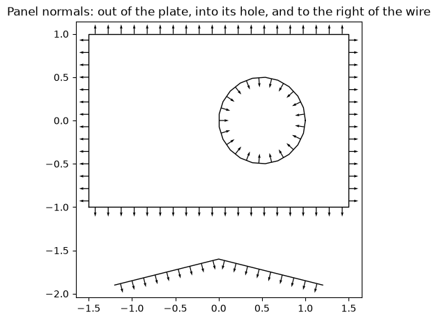

Crossing the boundary

A particle pusher moves each particle in a straight step, from its old to its new position. crossings(start, end) finds where each step first crosses the boundary, entering or leaving, for all steps at once: hit, the fraction of the step, the point and the unit normal pointing out of the region where contains is true. Because the whole step is tested, a fast particle cannot jump over a thin plate, or a wire, between its two end points. Polygons, circles, spheres, boxes and their transforms are exact; other shapes, Boolean ones included, are sampled along each step.

start = np.stack((np.full(12, -1.0), np.linspace(-1.15, 1.15, 12)))
end = start + np.array([[2.0], [0.0]])  # one long step each, across the slit
hits = slit.crossings(start, end)
hit = np.asarray(hits.hit)
print(f"{hit.sum()} of {hit.size} steps hit a plate")

fig, ax = plt.subplots(figsize=(5, 4), layout="constrained")
for loop in slit.outlines():
    ax.fill(*loop, color="0.8")
for i in range(start.shape[1]):
    ax.plot(
        [start[0, i], end[0, i]],
        [start[1, i], end[1, i]],
        color="C0" if hit[i] else "0.6",
    )
ax.plot(*np.asarray(hits.point)[:, hit], "o", color="C3", label="first crossing")
ax.set_aspect("equal")
ax.legend(loc="upper left", bbox_to_anchor=(1.02, 1.0))
plt.show()

through_the_gap = np.abs(start[1]) < 0.3
assert not hit[through_the_gap].any() and hit[~through_the_gap].all()
np.testing.assert_allclose(np.asarray(hits.point)[0, hit], -0.25)  # the front face

10 of 12 steps hit a plate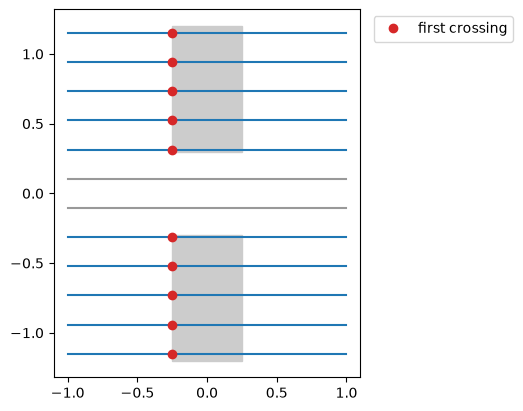

Try a graded spacing that refines the corners of the L-shaped polygon, where the field of a charged conductor is singular.