Conductors and level sets

Download notebookView on GitHubRun when the site was built.

Build an Einzel lens from ring electrodes, give the electrodes voltages, and read the Dirichlet values a field solver needs. The rings are Tube solids; their level sets locate the surface between grid nodes to round-off.

An Einzel lens is three coaxial rings: the outer two grounded, the middle one at a high voltage. A beam passing through the bore is focused without changing its final energy.

import matplotlib.pyplot as plt
import numpy as np

from simgeometry import GeometryCollection, Grid, Tube

bore, outer, length, gap = 1.0, 1.6, 0.8, 0.4


def ring(centre):
    # a ring electrode along z, with rounded edges
    return Tube(
        (0, 0, centre - length / 2),
        (0, 0, centre + length / 2),
        bore,
        outer,
        fillet=0.1,
    )


lens = GeometryCollection(
    {
        "entrance": ring(-(length + gap)),
        "focus": ring(0.0),
        "exit": ring(length + gap),
    },
    voltages={"entrance": 0.0, "focus": 10e3, "exit": 0.0},
)
print(lens.conductors, lens.voltages)

('entrance', 'focus', 'exit') {'entrance': 0.0, 'focus': 10000.0, 'exit': 0.0}

The section through the axis shows the three rings in the plane y = 0, labelled in insertion order.

lens.slice(y=0).show(resolution=240, display=False)
plt.title("Einzel lens, section y = 0")
plt.show()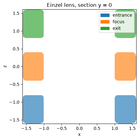

In 3D, color_by="voltage" colours each conductor by its voltage (needs simgeometry[interactive]); click Interactive 3-D view to look into the bore.

import plasma_plots
import pyvista as pv

pv.OFF_SCREEN = True
plotter = lens.show_3d(
    backend="pyvista", display=False, color_by="voltage", resolution=48, opacity=0.8
)
plasma_plots.scene(plotter, alt="The Einzel lens, the middle ring at 10 kV")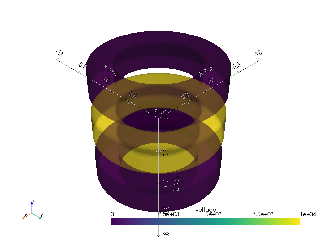

Interactive 3-D view (1.5 MB)Open in a new tab

Dirichlet values on a grid

dirichlet_values(grid) returns, for every node, the label of the object it is inside (0 outside every object) and that object’s voltage, NaN outside the conductors. Overlaps follow the labels: the last listed object wins. A solver fixes the nodes where values.conductor is true.

grid = Grid(
    ndim=3,
    lower_bound=(-2.0, -2.0, -3.0),
    upper_bound=(2.0, 2.0, 3.0),
    num_gridpoints=(41, 41, 61),
)
values = lens.dirichlet_values(grid)
print(values.names, values.labels.shape, int(values.conductor.sum()), "fixed nodes")

y0 = 20  # the node plane y = 0
x, _, z = grid.get_grid_points()
fig, ax = plt.subplots(figsize=(7, 3.5), layout="constrained")
image = ax.pcolormesh(
    z, x, values.voltages[:, y0, :], shading="nearest", cmap="viridis"
)
fig.colorbar(image, label="voltage [V]")
ax.set_xlabel("z")
ax.set_ylabel("x")
ax.set_aspect("equal")
ax.set_title("Dirichlet voltages at the nodes (white: free nodes)")
plt.show()

('entrance', 'focus', 'exit') (41, 41, 61) 11256 fixed nodes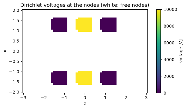

Other voltages without rebuilding the geometry

with_voltages returns a collection with the same objects and other voltages, for a parameter scan. A voltage can also be a function of the time t, such as a ramp; voltages_at(t) and dirichlet_values(..., t=t) evaluate it.

scan = {v: lens.with_voltages(focus=v) for v in (2e3, 5e3, 10e3)}
print({v: collection.voltages["focus"] for v, collection in scan.items()})

ramped = lens.with_voltages(focus=lambda t: 10e3 * min(t / 1e-6, 1.0))
for t in (0.0, 0.25e-6, 2e-6):
    print(f"t = {t:.2e} s:", ramped.voltages_at(t))
assert lens["focus"] is ramped["focus"]  # the same geometry

{2000.0: 2000.0, 5000.0: 5000.0, 10000.0: 10000.0}
t = 0.00e+00 s: {'entrance': 0.0, 'focus': 0.0, 'exit': 0.0}
t = 2.50e-07 s: {'entrance': 0.0, 'focus': 2500.0, 'exit': 0.0}
t = 2.00e-06 s: {'entrance': 0.0, 'focus': 10000.0, 'exit': 0.0}

Level sets

Analytic shapes have a level_set(points): negative inside, positive outside, zero on the boundary, the same sign as signed_distance. Where level_set_exact is true it is the Euclidean signed distance, so signed_distance returns it directly. Booleans combine level sets by minimum and maximum, which bounds the distance without being exact; transforms keep them exact for rigid motions and uniform scaling.

focus = lens["focus"]
points = np.array([[0.0, 1.3, 2.0], [0.0, 0.0, 0.0], [0.0, 0.0, 0.0]])
print("exact:", focus.level_set_exact)
print("level set:", focus.level_set(points))
print("signed distance:", focus.signed_distance(points))

exact: True
level set: [ 1.  -0.3  0.4]
signed distance: [ 1.  -0.3  0.4]

Cut a slot through the focus electrode and the level set becomes a bound. Below are its levels 0 (the surface) and 0.2 (a shell outside it); bounds leaves room for the shell. Where the shell dips into the slot it keeps sharp corners, where the shell of the exact distance would be rounded: the difference takes the maximum of two level sets. Click Interactive 3-D view and zoom into the slot.

from simgeometry import Cuboid

slotted = focus - Cuboid((0, 1.3, 0), (0.6, 1.0, 1.0))
print("exact:", slotted.level_set_exact)
field = slotted.level_set_field(resolution=64, bounds=((-2, -2, -0.8), (2, 2, 0.8)))
plotter = field.plasma.plot.isosurface(
    values=[0.0, 0.2], clim=(0.0, 0.3), opacity=0.5, show_domain=False
)
plotter.view_vector((0.5, 1, 0.8))  # look at the slot
plotter.camera.zoom(1.3)
plasma_plots.scene(
    plotter, alt="A ring electrode with a slot, and its level set 0.2 outside it"
)

exact: False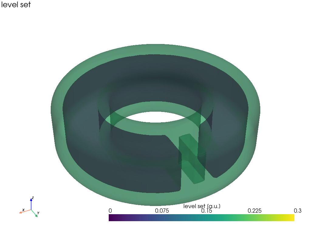

Interactive 3-D view (1.9 MB)Open in a new tab

Grid-edge crossings (bracketed_edge_geometry, used by Picnic’s embedded-boundary stencil) interpolate the level set between the two nodes of a cut edge and refine the root with a few Illinois steps, instead of bisecting contains 48 times. edges.points holds the crossings in world coordinates (edges.normals the outward normals there); they lie on the bore surface to round-off.

from simgeometry.cut_edges import bracketed_edge_geometry

edges = bracketed_edge_geometry(grid, [focus])
errors = np.abs(focus.level_set(edges.points))
print(
    f"{errors.size} cut edges, largest distance from the surface:",
    f"{errors.max():.1e}",
)

2640 cut edges, largest distance from the surface: 4.4e-16

edges.show_3d() draws the crossings over the translucent electrode: they trace the bore, the outer wall and the end faces; each one sits on a grid line. Click Interactive 3-D view and zoom in on an edge to see the crossings follow its rounding.

plotter = edges.show_3d(backend="pyvista", display=False, opacity=0.3, point_size=3)
plasma_plots.scene(
    plotter, alt="The grid-edge crossings on the surface of the focus electrode"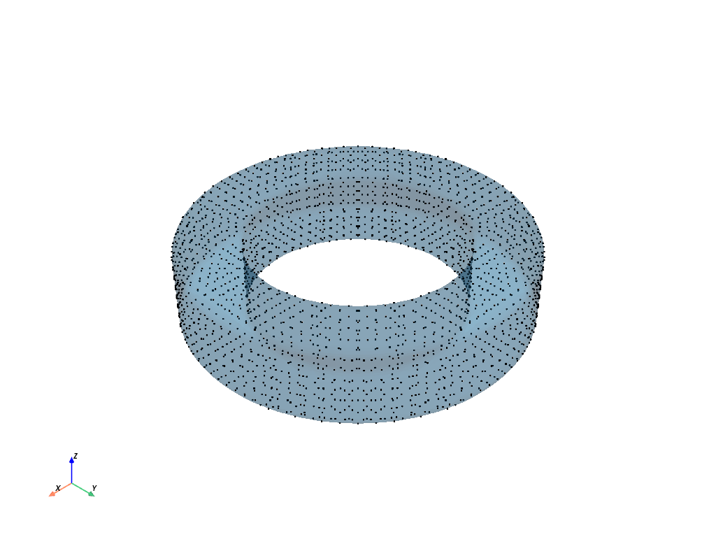
)

Interactive 3-D view (1.4 MB)Open in a new tab

Shapes known only through their membership, such as FunctionObject3D, have no level set (has_level_set is false); every query then falls back to sampling and bisecting contains.