Negative-ion beamlet optimisation
The second problem of beamtracer.optimization, after the einzel lens: one round H
beamlet extracted from a plasma, solved with BeamOptics and NegativeExtractionPlasma
(the beamlet of the example negative_ion_extraction_optics). The driver is unchanged:
the same Problem, scan and optimize, with NegativeIonBeamlet as the evaluation.
The design parameters are the extraction voltage, the aperture radius of the extraction grid (EG) and the gap from the plasma grid (PG) to the EG; the objective is the rms divergence of the H behind the grounded grid (GG), under the requirements of a beamlet for neutral beam injection: below 7 mrad, at about 300 A/m², with all of the H transmitted and the field on the grid surfaces below a voltage-holding limit.
This page solves a few designs live on a coarse mesh and loads the longer runs (the
searches, a comparison of the coarse mesh with the example’s, and the best designs solved
again on the example’s mesh) from records made with
tutorials/data/negative_ion_beamlet.py. The last part searches the full design: nine
parameters, the radii, thicknesses and gaps of the grids and the voltage split.
from pathlib import Path
import matplotlib.pyplot as pltimport numpy as np
from beamtracer.optimization import load_record, optimize, recheck, scanfrom beamtracer.optimization.beamlet import (    COARSE,    FULL_CONSTRAINTS,    FULL_DESIGN,    PARAMETERS,    NegativeIonBeamlet,)
BLUE, ORANGE, AQUA, YELLOW = "#2a78d6", "#eb6834", "#1baf7a", "#eda100"INK, MUTED, ELECTRODE = "#2b2a26", "#8a897f", "#b9b8b0"plt.rcParams.update(    {        "figure.dpi": 110,        "axes.edgecolor": MUTED,        "axes.labelcolor": INK,        "axes.grid": True,        "grid.color": "#e4e3dd",        "grid.linewidth": 0.6,        "xtick.color": MUTED,        "ytick.color": MUTED,        "legend.frameon": False,        "lines.linewidth": 2,    })WORKERS = 1  # processes for the live scanDATA = Path("data")  # the records of the longer runsBOUNDS = {    "extraction_voltage": (3e3, 10e3),    "eg_radius": (2e-3, 4e-3),    "gap": (3e-3, 6e-3),}
The beamlet
Section titled “The beamlet”NegativeIonBeamlet holds the fixed settings and builds the BeamOpticsConfig of a design.
Three grids in cylindrical geometry: the PG at 0 V with an 8 mm aperture and a
chamfer, the EG at the extraction voltage and the GG at 20 kV, the beam’s final energy; the
aperture edges of the EG and the GG are rounded, so that their surface field stays finite
as the mesh is refined. 300 A/m² of H and as much electron current leave the plasma,
whose positive ions follow a Boltzmann distribution and form the meniscus; a Vlasov
iteration converges the field and the trajectories together.
COARSE is the setting of the search: a 0.2 mm mesh and 100 trajectories per species,
against the example’s 0.1 mm and 300. One evaluation returns the divergence, the
constraints (<= 0 when met) and diagnostics:
beamlet = NegativeIonBeamlet(**COARSE)problem = beamlet.problem(BOUNDS)evaluation = problem.evaluate( {"extraction_voltage": 8e3, "eg_radius": 3e-3, "gap": 4e-3})d = evaluation.diagnosticsprint( f"divergence {evaluation.objectives['divergence'] * 1e3:.1f} mrad, " f"converged: {evaluation.converged} ({d['iterations']} iterations), " f"{evaluation.wall_time:.0f} s")print( f"transmission {d['transmission']:.1%}, extracted {d['current_density']:.0f} A/m², " f"energy {d['energy'] / 1e3:.1f} keV, J/J_CL {d['perveance_ratio']:.2f}")print( f"surface field: PG {d['field_pg'] / 1e6:.1f}, EG {d['field_eg'] / 1e6:.1f}, " f"GG {d['field_gg'] / 1e6:.1f} MV/m (limit {beamlet.field_limit / 1e6:.0f} MV/m on EG and GG)")print("constraints:", {k: round(v, 3) for k, v in evaluation.constraints.items()})divergence 27.6 mrad, converged: True (20 iterations), 4 stransmission 100.0%, extracted 271 A/m², energy 19.8 keV, J/J_CL 0.19surface field: PG 3.6, EG 2.4, GG 2.2 MV/m (limit 5 MV/m on EG and GG)constraints: {'loss': -0.01, 'surface_field': -0.519}The extracted current density is below 300 A/m² even with all of the H transmitted: it is the current over the whole PG aperture, and the beams start 0.2 mm inside its edge. The current density is an input of the steady model, set by the source; a design has to extract it at that perveance, which the loss constraint checks.
Unconverged solves
Section titled “Unconverged solves”Where the beam grazes the EG, or where the edge of the meniscus turns part of the H
back into the plasma, the Vlasov iteration does not settle: the potential keeps changing
by volts from one iteration to the next, in a limit cycle. Such an evaluation has
converged=False; the searches rank it behind every converged one, so it never wins, and
its diagnostics keep the spread of the divergence and the transmission over the last five
iterations. A scan over the extraction voltage at the default geometry:
voltages = np.linspace(3e3, 10e3, 8)swept = scan( problem, {"extraction_voltage": voltages, "eg_radius": [3e-3], "gap": [4e-3]}, workers=WORKERS,)print(" U_ex divergence spread transmission converged")for e in swept.evaluations: d = e.diagnostics print( f"{e.parameters['extraction_voltage'] / 1e3:4.0f} kV {e.objectives['divergence'] * 1e3:6.1f} mrad" f" {d['divergence_spread'] * 1e3:5.2f} {d['transmission']:9.1%} {e.converged}" ) U_ex divergence spread transmission converged 3 kV 15.8 mrad 0.00 70.1% True 4 kV 23.3 mrad 13.62 94.2% False 5 kV 17.3 mrad 7.42 98.1% False 6 kV 20.0 mrad 5.50 100.0% False 7 kV 23.8 mrad 0.01 100.0% True 8 kV 27.6 mrad 0.01 100.0% True 9 kV 30.7 mrad 0.00 100.0% True 10 kV 33.4 mrad 0.00 100.0% Truefig, ax = plt.subplots(figsize=(7, 3.6))v = np.array([e.parameters["extraction_voltage"] for e in swept.evaluations]) / 1e3div = np.array([e.objectives["divergence"] for e in swept.evaluations]) * 1e3spread = np.array([e.diagnostics["divergence_spread"] for e in swept.evaluations]) * 1e3ok = np.array([e.converged for e in swept.evaluations])ax.plot(v, div, color=MUTED, lw=1)ax.errorbar( v[~ok], div[~ok], yerr=spread[~ok] / 2, fmt="x", color=ORANGE, ms=8, capsize=3, label="not converged (bar: spread over the last iterations)",)ax.scatter(v[ok], div[ok], color=BLUE, s=36, zorder=3, label="converged")ax.axhline(7, color=INK, ls="--", lw=1, label="7 mrad")ax.set_xlabel("extraction voltage [kV]")ax.set_ylabel("rms divergence of the H$^-$ [mrad]")ax.set_ylim(0, None)ax.legend(fontsize=8)fig.tight_layout()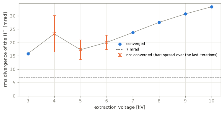
The coarse mesh against the example’s
Section titled “The coarse mesh against the example’s”The example’s setting (0.1 mm, 300 trajectories per species) takes 10 to 20 s per solve
on one core here, the coarse one 4 to 10 s. Eight designs spread over the search space,
solved with both (tutorials/data/negative_ion_beamlet.py resolution):
fine = load_record(DATA / "beamlet_resolution_fine.jsonl")coarse = load_record(DATA / "beamlet_resolution_coarse.jsonl")print( " U_ex r_EG gap | fine: div transm. conv. | coarse: div transm. conv. | difference")for k in range(fine.sizes["evaluation"]): f, c = fine.isel(evaluation=k), coarse.isel(evaluation=k) both = bool(f.converged) and bool(c.converged) change = f"{float(c.divergence / f.divergence - 1):+.1%}" if both else "-" print( f"{float(f.extraction_voltage) / 1e3:5.2f} {float(f.eg_radius) * 1e3:5.2f} {float(f.gap) * 1e3:5.2f} | " f"{float(f.divergence) * 1e3:9.1f} {float(f.transmission):8.1%} {'yes' if f.converged else 'no':>5} | " f"{float(c.divergence) * 1e3:11.1f} {float(c.transmission):8.1%} {'yes' if c.converged else 'no':>5} | {change}" )print( f"wall time per solve: fine {float(fine.wall_time.mean()):.0f} s, " f"coarse {float(coarse.wall_time.mean()):.0f} s") U_ex r_EG gap | fine: div transm. conv. | coarse: div transm. conv. | difference 3.80 2.19 5.33 | 6.3 29.9% yes | 13.2 32.4% yes | +109.0% 6.87 3.98 5.84 | 21.8 95.2% no | 19.0 100.0% no | - 5.21 3.71 4.22 | 19.4 89.5% no | 17.3 100.0% no | - 6.40 2.65 5.06 | 22.3 88.0% no | 21.0 83.4% no | - 4.37 2.35 3.85 | 20.0 79.2% no | 18.2 73.6% no | - 8.29 3.43 3.51 | 29.8 100.0% yes | 29.7 100.0% yes | -0.4% 7.64 3.18 3.37 | 28.8 100.0% yes | 28.6 100.0% yes | -0.7% 9.15 2.93 4.76 | 28.8 100.0% yes | 28.3 100.0% yes | -1.6%wall time per solve: fine 29 s, coarse 13 sWhere both settings converge with all of the H transmitted, the coarse divergence is within 2 % of the fine one (0.4 to 1.6 % lower), at less than half the cost. Where the EG scrapes the beam (the first design, 30 % transmitted) they differ by a factor of two: the divergence of a scraped beam depends on which trajectories survive, and the loss constraint excludes such designs anyway. The other four designs converge on neither mesh: the limit cycle belongs to the model at these designs, not to the coarse mesh, and the coarse mesh flags the same designs. So the coarse setting is honest where the search uses it; but the edge of the region where the iteration converges moves with the mesh, and that is where the optimum lies (below).
The search
Section titled “The search”Differential evolution on the coarse mesh with a small budget (population 5 per
parameter, 8 generations, two workers), minimizing the divergence with the loss and the
surface field as constraints (tutorials/data/negative_ion_beamlet.py search). Its record:
search = load_record(DATA / "beamlet_search.jsonl")feasible = search.feasible.valuesbest = int(np.argmin(np.where(feasible, search.divergence.values, np.inf)))b = search.isel(evaluation=best)print( f"{search.sizes['evaluation']} evaluations: {int(search.converged.sum())} converged, " f"{int(feasible.sum())} feasible; " f"{float(search.wall_time.sum()) / 3600:.1f} h of solves, " f"{float(search.wall_time.mean()):.0f} s each")print( f"best: U_ex {float(b.extraction_voltage) / 1e3:.2f} kV, r_EG {float(b.eg_radius) * 1e3:.2f} mm, " f"gap {float(b.gap) * 1e3:.2f} mm: divergence {float(b.divergence) * 1e3:.1f} mrad, " f"transmission {float(b.transmission):.1%}, EG field {float(b.field_eg) / 1e6:.1f} MV/m")135 evaluations: 78 converged, 62 feasible; 0.4 h of solves, 10 s eachbest: U_ex 6.14 kV, r_EG 3.78 mm, gap 3.72 mm: divergence 20.9 mrad, transmission 100.0%, EG field 2.2 MV/mfig, axes = plt.subplots(1, 2, figsize=(10, 3.8))ax = axes[0]v = search.extraction_voltage.values / 1e3div = search.divergence.values * 1e3converged = search.converged.valuesfor mask, color, marker, label in ( (feasible, BLUE, "o", "feasible"), (converged & ~feasible, YELLOW, "s", "converged, H$^-$ lost"), (~converged, ORANGE, "x", "not converged"),): ax.scatter( v[mask], div[mask], s=18, color=color, marker=marker, label=label, alpha=0.8 )ax.scatter( v[best], div[best], s=200, marker="*", color=INK, edgecolor="white", zorder=4, label="best",)ax.axhline(7, color=INK, ls="--", lw=1)ax.set_xlabel("extraction voltage [kV]")ax.set_ylabel("rms divergence [mrad]")ax.legend(fontsize=8)ax = axes[1]r = search.eg_radius.values * 1e3gap = search.gap.values * 1e3for mask, color, marker in ( (feasible, BLUE, "o"), (converged & ~feasible, YELLOW, "s"), (~converged, ORANGE, "x"),): ax.scatter(r[mask], gap[mask], s=18, color=color, marker=marker, alpha=0.8)ax.scatter( r[best], gap[best], s=200, marker="*", color=INK, edgecolor="white", zorder=4)ax.set_xlabel("EG aperture radius [mm]")ax.set_ylabel("PG-EG gap [mm]")fig.tight_layout()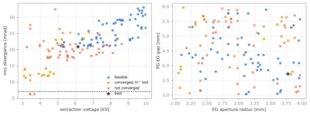
The feasible designs (converged, all of the H transmitted) have 21 to 33 mrad: the requirement of 7 mrad is out of reach in this design space, and divergences below 10 mrad appear only where the EG scrapes a third of the beam or more. The divergence falls with the extraction voltage, as the meniscus becomes less concave and over-focuses less, until the iteration stops converging, near 6 kV: the optimum sits on the edge of the region where the solve converges, with a wide EG aperture and a short gap. The surface fields stay far below the 5 MV/m limit, which is not active.
The best design on the example’s mesh, solved live (iterates collects the H moments
of every Vlasov iteration, from which the evaluation takes the spread over the last ones):
design = {name: float(b[name]) for name in ("extraction_voltage", "eg_radius", "gap")}fine_beamlet = NegativeIonBeamlet(save_trajectories=4)iterates = [] # the H- moments of every Vlasov iterationmodel = fine_beamlet.solve(design, iterates=iterates)check = fine_beamlet.at(design).measure(model, iterates)print( f"fine mesh: divergence {check.objectives['divergence'] * 1e3:.1f} mrad " f"(coarse {float(b.divergence) * 1e3:.1f}), converged: {check.converged}, " f"spread over the last iterations {check.diagnostics['divergence_spread'] * 1e3:.1f} mrad, " f"potential change {check.diagnostics['potential_change']:.2f} V")fine mesh: divergence 24.9 mrad (coarse 20.9), converged: False, spread over the last iterations 0.1 mrad, potential change 0.05 Vpotential = model.potential_field.evaluate()fig, ax = plt.subplots(figsize=(10, 3.4))mesh = ax.pcolormesh( potential.x * 1e3, potential.y * 1e3, potential.T / 1e3, cmap="Blues", shading="auto",)fig.colorbar(mesh, ax=ax, label="potential [kV]", pad=0.01)for params in model.config.objects.values(): for loop in params.build().outlines(): ax.fill( loop[0] * 1e3, np.minimum(loop[1], fine_beamlet.radius) * 1e3, color=ELECTRODE, lw=0, )for path, species in zip(model.trajectories, model.trajectory_species, strict=True): if species == 0: ax.plot(path[:, 0] * 1e3, path[:, 1] * 1e3, color=ORANGE, lw=0.6)ax.set_ylim(0, fine_beamlet.radius * 1e3)ax.set_xlabel("x [mm]")ax.set_ylabel("r [mm]")ax.set_title( "the best design on the fine mesh: every 4th H$^-$ trajectory", color=INK, fontsize=10,)ax.grid(False)fig.tight_layout()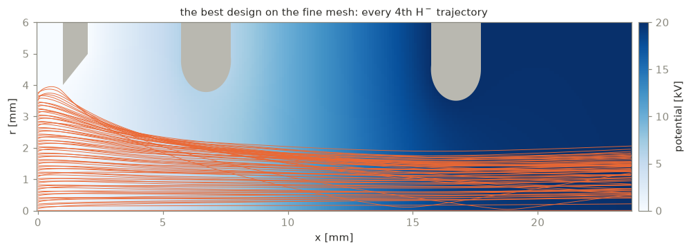
On the example’s mesh the best design reaches 24.9 mrad, 19 % above its coarse value, and does not meet the tolerance within 40 iterations: its potential still changes by 0.05 V per iteration and its divergence by 0.1 mrad, a slow approach rather than a limit cycle of volts, which the search still counts as unconverged. Near the edge of the convergent region the coarse mesh is much less accurate than in the comparison above. A design from the coarse search has to be checked at the fine setting, and the few best rather than the best alone, since the best is the one closest to that edge.
Checking the best designs
Section titled “Checking the best designs”recheck takes a search’s result and evaluates its best few designs (by the search’s
ranking: feasible ones first, never a failed or unconverged one) with another
evaluation: here the same beamlet on the example’s mesh, in general any function of the
design’s configuration that returns an Evaluation. The search’s result comes from its
record (optimize with the same seed resumes it without a new solve), and the check’s
evaluations from theirs:
search_result = optimize( NegativeIonBeamlet(**COARSE).problem(BOUNDS), seed=1, popsize=5, maxiter=8, record=DATA / "beamlet_search.jsonl",)checked = recheck( search_result, NegativeIonBeamlet().problem(BOUNDS), top=5, workers=WORKERS, record=DATA / "beamlet_search_fine.jsonl",)print( f"search resumed: {search_result.evaluated} new solves; check: {checked.evaluated} new solves")print(" U_ex r_EG gap | coarse | fine converged transmission")coarse_of = { search_result.problem.design.key(e.parameters): e for e in search_result.evaluations}for e in checked.evaluations: c = coarse_of[search_result.problem.design.key(e.parameters)] p = e.parameters print( f"{p['extraction_voltage'] / 1e3:5.2f} {p['eg_radius'] * 1e3:5.2f} {p['gap'] * 1e3:5.2f} | " f"{c.objectives['divergence'] * 1e3:5.1f} | {e.objectives['divergence'] * 1e3:5.1f} " f"{'yes' if e.converged else 'no':>5} {e.diagnostics['transmission']:10.1%}" )if checked.best is not None and checked.best.feasible: print(f"best on the fine mesh: {checked.fun * 1e3:.1f} mrad at {checked.x}")search resumed: 0 new solves; check: 0 new solves U_ex r_EG gap | coarse | fine converged transmission 6.14 3.78 3.72 | 20.9 | 24.9 no 100.0% 5.35 3.66 3.16 | 20.9 | 28.1 no 100.0% 5.28 3.65 3.11 | 20.9 | 25.1 no 100.0% 7.56 3.05 4.94 | 20.9 | 25.5 no 100.0% 5.28 3.16 3.11 | 21.1 | 24.2 no 100.0%None of the five best designs of the search converges on the example’s mesh: all lie near the edge of the convergent region, and on the fine mesh they read 24 to 28 mrad, 15 to 35 % above their coarse values. The three-parameter search found no design that holds on the fine mesh, and the check says so instead of passing on a coarse optimum.
The full design
Section titled “The full design”Nine parameters: the extraction voltage (the split of the 20 kV between the gaps), the
three aperture radii, the three grid thicknesses and the two gaps (FULL_DESIGN), with
voltage holding as constraints (FULL_CONSTRAINTS): the largest field on the EG and GG
surfaces below 5 MV/m, and the mean field of each gap (its voltage over its length) below
3 MV/m. The domain radius, half the pitch of the beamlets, stays 6 mm: a design whose
apertures do not fit is a failed evaluation. The search on the coarse mesh has a small
budget (population 3 per parameter, 5 generations); the check solves its best five
designs on the example’s mesh.
full = load_record(DATA / "beamlet_full_design.jsonl")ok = full.ok.valuesfeasible_full = full.feasible.valuesfailed = full.failure.values != ""print( f"{full.sizes['evaluation']} evaluations: {int(failed.sum())} could not be built, " f"{int((~ok & ~failed).sum())} did not converge, {int(feasible_full.sum())} feasible; " f"{float(full.wall_time.sum()) / 3600:.1f} h of solves")full_result = optimize( NegativeIonBeamlet(**COARSE).problem(FULL_DESIGN, FULL_CONSTRAINTS), seed=1, popsize=3, maxiter=5, record=DATA / "beamlet_full_design.jsonl",)full_checked = recheck( full_result, NegativeIonBeamlet().problem(FULL_DESIGN, FULL_CONSTRAINTS), top=5, workers=WORKERS, record=DATA / "beamlet_full_design_fine.jsonl",)names = list(PARAMETERS)units = {"V": 1e-3, "m": 1e3}print("".join(f"{name[:12]:>13}" for name in names) + " coarse fine converged")coarse_of = { full_result.problem.design.key(e.parameters): e for e in full_result.evaluations}for e in full_checked.evaluations: c = coarse_of[full_result.problem.design.key(e.parameters)] row = "".join(f"{e.parameters[n] * units[PARAMETERS[n]]:13.2f}" for n in names) print( f"{row} {c.objectives['divergence'] * 1e3:6.1f} {e.objectives['divergence'] * 1e3:6.1f}" f" {'yes' if e.converged else 'no':>5}" )print("(kV and mm; divergence in mrad)")162 evaluations: 9 could not be built, 65 did not converge, 70 feasible; 1.3 h of solves extraction_v eg_radius gap pg_radius gg_radius pg_thickness eg_thickness gg_thickness acceleration coarse fine converged 6.49 2.78 4.59 3.60 3.70 0.58 2.43 1.36 8.48 19.9 22.2 no 6.06 2.55 4.16 3.43 3.50 0.57 2.47 1.39 8.51 20.6 22.3 yes 5.64 2.73 4.02 3.93 3.51 0.52 2.19 1.08 6.60 20.9 22.0 yes 7.09 2.72 5.09 3.89 2.75 0.58 1.48 1.90 7.98 21.0 22.5 yes 6.49 2.60 3.67 4.15 3.66 1.29 2.43 1.36 8.48 21.0 24.0 no(kV and mm; divergence in mrad)The full design does a little better on the coarse mesh (19.9 mrad against 20.9) and, more usefully, three of its five best designs converge on the example’s mesh, where the best reaches 22.0 mrad, 5 % above its coarse value: 5.6 kV across a 4.0 mm gap, a thin PG (0.5 mm) with a 3.9 mm aperture, a 2.7 mm EG aperture in a 2.2 mm thick EG, and a 6.6 mm acceleration gap. The thin PG and the thick EG recur among the best designs. Neither voltage-holding limit is active there (3.4 MV/m on the grid surfaces, 2.2 MV/m in the acceleration gap). The result is still far from 7 mrad, and the search is only a sample of the nine-dimensional space: 162 evaluations, a population of 27 for five generations. The full run in the next section (population 15 per parameter, 100 generations) needs about 14 000 solves, some 40 core-hours at 10 s per coarse solve.
A check by a PIC model
Section titled “A check by a PIC model”The check is a function of what the design builds, here the NegativeIonBeamlet of a
design (its geometry, voltages and beams), so a time-dependent PIC model of the source
plugs in from user code, and beamtracer never imports it. The function must be defined in
a module (not in a notebook) for worker processes, and return the objectives and the
constraints of the search’s problem:
from beamtracer.optimization import Evaluation

def pic_check(beamlet):    run = my_pic_code.beamlet(  # any model: picnic, another code, a measurement        pg_radius=beamlet.pg_radius, eg=beamlet.eg, gg=beamlet.gg, ...    )    return Evaluation(        objectives={"divergence": run.rms_angle},        constraints={            "loss": run.lost_fraction - beamlet.max_loss,            "surface_field": run.surface_field / beamlet.field_limit - 1.0,            "gap_field": max(beamlet.gap_fields.values()) / beamlet.gap_field_limit - 1.0,        },        converged=run.settled,        diagnostics={"electron_ratio": run.electron_ratio},    )
from beamtracer.optimization import recheckfrom my_checks import pic_check
checked = recheck(full_result, pic_check, top=3, workers=2, record="pic.jsonl")Running the search yourself
Section titled “Running the search yourself”The problem pickles (a frozen dataclass), so the searches run it in worker processes; the
record makes a search resumable. With timeout, a solve that hangs becomes a failed
evaluation:
from beamtracer.optimization import optimize, recheckfrom beamtracer.optimization.beamlet import (    COARSE, FULL_CONSTRAINTS, FULL_DESIGN, NegativeIonBeamlet)
problem = NegativeIonBeamlet(**COARSE).problem(    FULL_DESIGN, FULL_CONSTRAINTS + ("divergence_limit",)  # the 7 mrad as a constraint)result = optimize(    problem, seed=1, popsize=15, maxiter=100, workers=-1, record="beamlet.jsonl", timeout=600)checked = recheck(    result, NegativeIonBeamlet().problem(FULL_DESIGN, FULL_CONSTRAINTS), top=10, workers=-1)
The records of this page come from python tutorials/data/negative_ion_beamlet.py; its
full step takes --popsize, --maxiter and --workers for a longer search.