Calorimeter

Download notebook View on GitHubRun when the site was built.

In a test facility the beam ends on a calorimeter: a plate of tiles whose temperature rise gives the power on each. From the map the experiments infer the beam’s width (a Gaussian fit of the footprint) and, from the widths at several distances or against the size of the grid, its divergence. Calorimeter records such a map from the markers, and fit_footprint and divergence_from_widths repeat the analysis, so the inferred divergence can be set against the markers’ own rms angle.

The beam is the group of 5 by 16 beamlets of the grid tutorial, each a Gaussian beamlet of 5 mrad.

import numpy as np
import plasma_plots as pp
import xarray as xr
from scipy import constants

from beamtracer.beamline import (
    ApertureGrid,
    Calorimeter,
    divergence_from_widths,
    fit_footprint,
    gaussian_beam,
)

mass = 2.014 * constants.atomic_mass
speed = np.sqrt(2 * 1e6 * constants.e / mass)
beamlet = gaussian_beam(2000, power=1e4, speed=speed, width=2e-3, divergence=5e-3)
flat = ApertureGrid.regular(16, 5, (0.020, 0.022)).markers(beamlet)
print(
    f"{len(flat)} markers, {flat.total_power / 1e6:.1f} MW, "
    f"rms angle of the markers {flat.rms_angle * 1e3} mrad"
)

160000 markers, 0.8 MW, rms angle of the markers [4.9481817  5.11957346] mrad

The maps

The calorimeter, 0.8 m square in 2 cm tiles, at 3, 5 and 7 m from the grid. Close to the grid the footprint is the group’s rectangle blurred by the beamlets; further away it rounds.

distances = (3.0, 5.0, 7.0)
maps = [
    Calorimeter(d, (-0.4, 0.4, -0.4, 0.4), (40, 40)).measure(flat) for d in distances
]
with pp.figure(1, 3, figsize=(12, 3.8)) as fig:
    for k, (d, power_map) in enumerate(zip(distances, maps, strict=True)):
        (power_map / 1e6).assign_attrs(units="MW/m²").plasma.plot.slice(
            x="y",
            y="z",
            equal_aspect=True,
            ax=fig[k],
            title=f"x = {d} m",
            colorbar_label="MW/m²",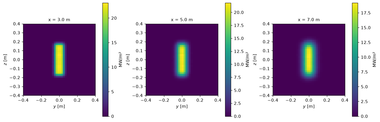
        )

The fit

A 2D Gaussian fitted to each map, and its profile through the centre against the map’s ( $z = 0$ , along $y$ ; and $y = 0$ , along $z$ ):

fits = [fit_footprint(power_map) for power_map in maps]
for d, fit in zip(distances, fits, strict=True):
    print(
        f"x = {d} m: width {fit['width_y'] * 1e3:.1f} mm in y, "
        f"{fit['width_z'] * 1e3:.1f} mm in z"
    )

power_map, fit = maps[-1], fits[-1]
with pp.figure(1, 2, figsize=(10, 3.6)) as fig:
    for k, (along, width) in enumerate((("y", "width_y"), ("z", "width_z"))):
        other = "z" if along == "y" else "y"
        centre = fit[f"centre_{along}"]
        profile = (power_map / 1e6).assign_attrs(
            units="MW/m²", long_name="power density"
        )
        profile.plasma.plot.lineout(
            x=along,
            ax=fig[k],
            reference=lambda s, c=centre, w=fit[width]: (
                fit["peak"] / 1e6 * np.exp(-0.5 * ((s - c) / w) ** 2)
            ),
            **{other: 0.0},
        )
        fig[k].set_title(f"x = 7 m, along {along}")
        fig[k].legend(["the map", "the Gaussian fit"], fontsize=8)

x = 3.0 m: width 37.2 mm in y, 126.1 mm in z
x = 5.0 m: width 40.8 mm in y, 126.8 mm in z
x = 7.0 m: width 46.6 mm in y, 127.9 mm in z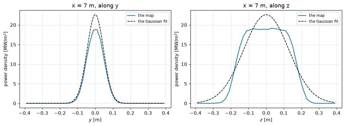

The group is 0.08 m wide in $y$ and 0.33 m in $z$ : in $z$ its flat top is still visible at 7 m and the Gaussian fits it only roughly.

The divergence

The widths against the distance, fitted with $w^2 = w_0^2 + (L\theta)^2$ :

rows = []
for direction in ("y", "z"):
    widths = [fit[f"width_{direction}"] for fit in fits]
    w0, theta = divergence_from_widths(distances, widths)
    rows.append((direction, w0, theta))
    print(f"in {direction}: w0 {w0 * 1e3:.0f} mm, divergence {theta * 1e3:.2f} mrad")
print(
    f"the markers: {flat.rms_angle[0] * 1e3:.2f} mrad in y, {flat.rms_angle[1] * 1e3:.2f} in z"
)

in y: w0 34 mm, divergence 4.46 mrad
in z: w0 126 mm, divergence 3.38 mrad
the markers: 4.95 mrad in y, 5.12 in z

For a flat grid every beamlet keeps its axis, so the spread of the slopes is the beamlet’s, 5 mrad. The analysis of the maps gets close to it in $y$ , where the group is narrow (4.5 mrad, 10 % low), and far below it in $z$ (3.4 mrad): the group’s flat top makes the fitted Gaussian too wide at short distances, and its width grows more slowly than the beam’s rms width, so the fit’s $w_0$ takes up part of the growth. This is the bias of the experiments’ analysis when the footprint is far from Gaussian, which the markers make visible.

A curved grid

Curved to 7 m, the beamlets converge: the slopes now include the aim, and the rms angle of the markers grows, while the footprint shrinks with the distance. The fit of the widths no longer measures a divergence:

curved = ApertureGrid.regular(16, 5, (0.020, 0.022), focal_length=(7.0, 7.0)).markers(
    beamlet
)
widths = xr.DataArray(
    [
        [
            fit_footprint(
                Calorimeter(d, (-0.4, 0.4, -0.4, 0.4), (40, 40)).measure(curved)
            )[f"width_{a}"]
            for d in np.linspace(1.0, 9.0, 9)
        ]
        for a in ("y", "z")
    ],
    dims=("direction", "x"),
    coords={
        "direction": ["y", "z"],
        "x": ("x", np.linspace(1.0, 9.0, 9), {"units": "m"}),
    },
    name="width",
    attrs={"units": "m", "long_name": "fitted width"},
)
with pp.figure(figsize=(7, 3.4)) as fig:
    for k in range(2):
        widths.plasma.plot.lineout(x="x", direction=k, ax=fig[0])
    fig[0].legend(["in y", "in z"], fontsize=8)
print(f"the markers' rms angle: {curved.rms_angle * 1e3} mrad (beamlet: 5 mrad)")

the markers' rms angle: [ 6.3888788  15.36653616] mrad (beamlet: 5 mrad)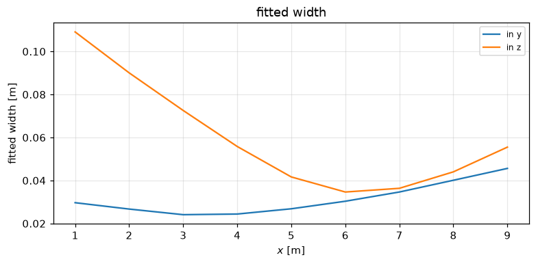

The fitted width falls to the focus at 7 m and grows beyond it: the beamlet divergence shows only near the focus, where the width is that of one beamlet, $\sqrt{w^2 + (7\,\mathrm{m} \cdot 5\,\mathrm{mrad})^2} \approx 35$ mm. This is why the experiments measure the divergence on a single beamlet group with a known aim, or at the focus.