Einzel lens design map

Optimising an einzel lens: the map and the optimiser’s path.

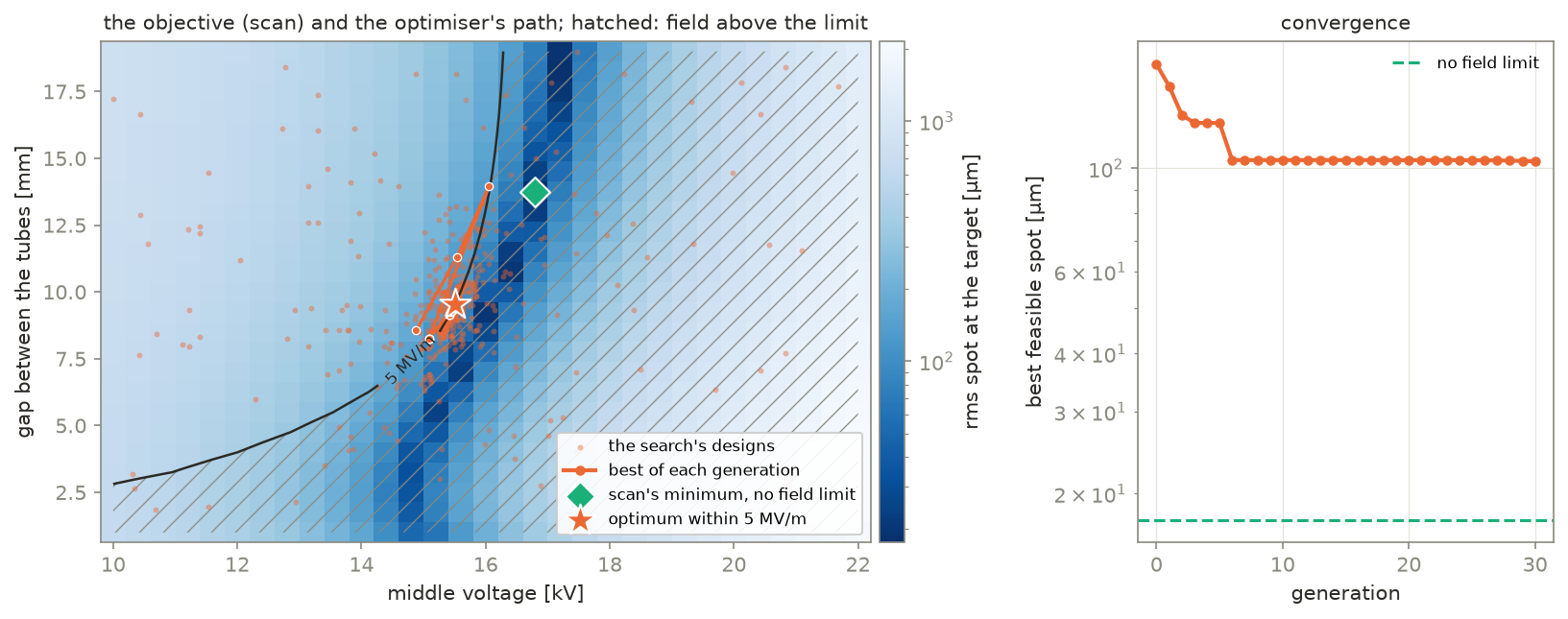
The einzel lens of beamtracer.optimization.einzel (the tutorial “Einzel lens optimisation”) with two parameters, the voltage of the middle tube and the gap between the tubes, and a limit of 5 MV/m on the field at the electrode surfaces. 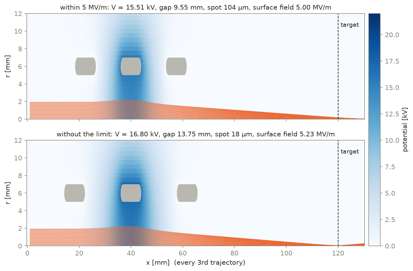A scan over a grid of designs maps the objective, the rms spot of a 30 keV proton beam at the target plane, and differential evolution searches the same problem; its path, the best design of each generation, is drawn over the map. The last plot is the lens it finds, and the scan’s best lens without the limit, with the trajectories over the potential.

The spot is smallest along a narrow valley, about 1 kV wide: the voltage that focuses on the target, which rises with the gap. The surface field rises with the voltage and falls with the gap up to about 12 mm, then hardly changes, while the valley keeps moving to higher voltages. So the 5 MV/m limit cuts the valley off at every gap, and the optimum is the point of the limit closest to the valley: 15.51 kV and a 9.55 mm gap, a 104 µm spot at 5.00 MV/m (near the 9.6 to 10 mm gaps of the tutorial’s three-parameter searches, whose bore is narrower). On the scan without the limit the smallest spot is 17.6 µm, at 16.8 kV and a 13.75 mm gap, with 5.23 MV/m: 5 % more field gives a six times smaller spot, because the focus moves through the target within a few hundred volts. The lens within the limit focuses beyond the target.

The search, population 20 for 30 generations with its first population spread over the whole map, closes in on the limit in the first six generations and then creeps along it.

Every evaluation is in the record examples/data/einzel_lens_design_map.jsonl, and the scan and the search take their designs from it instead of solving them again, so the page builds in seconds. Delete the record to solve everything again: about 1400 solves of a second each, WORKERS=4 python examples/einzel_lens_design_map.py runs them in four processes. The record knows only the parameters, not the fixed settings of the lens, so delete it too after changing those.

Python source

"""Einzel lens design map.

Optimising an einzel lens: the map and the optimiser's path.

The einzel lens of `beamtracer.optimization.einzel` (the tutorial "Einzel lens
optimisation") with two parameters, the voltage of the middle tube and the gap between the tubes,
and a limit of 5 MV/m on the field at the electrode surfaces. A scan over a grid of designs
maps the objective, the rms spot of a 30 keV proton beam at the target plane, and
differential evolution searches the same problem; its path, the best design of each
generation, is drawn over the map. The last plot is the lens it finds, and the scan's best
lens without the limit, with the trajectories over the potential.

The spot is smallest along a narrow valley, about 1 kV wide: the voltage that focuses on
the target, which rises with the gap. The surface field rises with the voltage and falls
with the gap up to about 12 mm, then hardly changes, while the valley keeps moving to higher
voltages. So the 5 MV/m limit cuts the valley off at every gap, and the optimum is the point
of the limit closest to the valley: 15.51 kV and a 9.55 mm gap, a 104 µm spot at 5.00 MV/m
(near the 9.6 to 10 mm gaps of the tutorial's three-parameter searches, whose bore is
narrower). On the scan without the limit the smallest spot is 17.6 µm, at 16.8 kV and a
13.75 mm gap, with 5.23 MV/m: 5 % more field gives a six times smaller spot, because the
focus moves through the target within a few hundred volts. The lens within the limit
focuses beyond the target.

The search, population 20 for 30 generations with its first population spread over the
whole map, closes in on the limit in the first six generations and then creeps along it.

Every evaluation is in the record `examples/data/einzel_lens_design_map.jsonl`, and the scan
and the search take their designs from it instead of solving them again, so the page builds
in seconds. Delete the record to solve everything again: about 1400 solves of a second each,
`WORKERS=4 python examples/einzel_lens_design_map.py` runs them in four processes. The
record knows only the parameters, not the fixed settings of the lens, so delete it too after
changing those.
"""

import os
from dataclasses import replace
from pathlib import Path

import matplotlib.pyplot as plt
import numpy as np
from matplotlib.colors import LogNorm

from beamtracer.optimization import optimize, scan
from beamtracer.optimization.einzel import EinzelLens

BLUE, ORANGE, AQUA = "#2a78d6", "#eb6834", "#1baf7a"
INK, MUTED, ELECTRODE = "#2b2a26", "#8a897f", "#b9b8b0"
plt.rcParams.update(
    {
        "figure.dpi": 110,
        "axes.edgecolor": MUTED,
        "axes.labelcolor": INK,
        "xtick.color": MUTED,
        "ytick.color": MUTED,
        "legend.frameon": False,
        "lines.linewidth": 2,
        "hatch.color": MUTED,
        "hatch.linewidth": 0.6,
    }
)
# Processes for the evaluations that are not in the record (1: none, in this process).
WORKERS = int(os.environ.get("WORKERS", "1"))
RECORD = Path(__file__).resolve().parent / "data" / "einzel_lens_design_map.jsonl"
BOUNDS = {"voltage": (10e3, 22e3), "gap": (1e-3, 19e-3)}
POPSIZE, MAXITER, SEED = 10, 30, 1


def main() -> None:
    """Scan, search and plot."""
    lens = EinzelLens()  # 30 keV protons, 2 mm beam, 5 mm bore, 0.5 mm mesh, 5 MV/m
    problem = lens.problem(BOUNDS, constraints=("loss", "surface_field"))
    RECORD.parent.mkdir(exist_ok=True)

    # The map: every design of a grid, 400 V by 0.75 mm.
    voltages = np.linspace(*BOUNDS["voltage"], 31)
    gaps = np.linspace(*BOUNDS["gap"], 25)
    grid = scan(
        problem, {"voltage": voltages, "gap": gaps}, workers=WORKERS, record=RECORD
    )
    shape = (len(voltages), len(gaps))  # the last parameter varies fastest
    spot = np.array([e.objectives["spot"] for e in grid.evaluations]).reshape(shape)
    field = np.array([e.diagnostics["field"] for e in grid.evaluations]).reshape(shape)
    lost = np.array([e.constraints["loss"] > 0 for e in grid.evaluations]).reshape(
        shape
    )
    free = np.unravel_index(np.nanargmin(np.where(lost, np.nan, spot)), shape)

    # The search, and its path: the best design of the initial population and after
    # each generation.
    search = optimize(
        problem,
        seed=SEED,
        popsize=POPSIZE,
        maxiter=MAXITER,
        tol=1e-6,
        workers=WORKERS,
        record=RECORD,
    )
    path = search.path
    generations = len(path)
    print(
        f"scan: {len(grid.evaluations)} designs, {grid.evaluated} solved; "
        f"search: {generations - 1} generations, {len(search.evaluations)} designs, "
        f"{search.evaluated} solved"
    )
    best = search.best
    print(
        f"optimum: V = {search.x['voltage'] / 1e3:.2f} kV, gap {search.x['gap'] * 1e3:.2f} mm, "
        f"spot {search.fun * 1e6:.1f} um, field {best.diagnostics['field'] / 1e6:.2f} MV/m"
    )
    print(
        f"scan without the field limit: V = {voltages[free[0]] / 1e3:.2f} kV, "
        f"gap {gaps[free[1]] * 1e3:.1f} mm, spot {spot[free] * 1e6:.1f} um, "
        f"field {field[free] / 1e6:.2f} MV/m"
    )

    # The map and the path.
    fig, (ax, conv) = plt.subplots(
        1, 2, figsize=(11, 4.4), gridspec_kw={"width_ratios": [2.2, 1]}
    )
    mesh = ax.pcolormesh(
        voltages / 1e3,
        gaps * 1e3,
        spot.T * 1e6,
        norm=LogNorm(vmin=np.nanmin(spot) * 1e6, vmax=np.nanmax(spot) * 1e6),
        cmap="Blues_r",
        shading="nearest",
        rasterized=True,
    )
    fig.colorbar(mesh, ax=ax, label="rms spot at the target [µm]", pad=0.01)
    ax.contourf(
        voltages / 1e3,
        gaps * 1e3,
        field.T,
        levels=[lens.field_limit, np.inf],
        colors="none",
        hatches=["//"],
    )
    limit = ax.contour(
        voltages / 1e3,
        gaps * 1e3,
        field.T,
        levels=[lens.field_limit],
        colors=INK,
        linewidths=1.2,
    )
    ax.clabel(limit, fmt={lens.field_limit: "5 MV/m"}, fontsize=8)
    v = np.array([e.parameters["voltage"] for e in search.evaluations]) / 1e3
    g = np.array([e.parameters["gap"] for e in search.evaluations]) * 1e3
    ax.scatter(v, g, s=8, color=ORANGE, alpha=0.45, lw=0, label="the search's designs")
    pv = np.array([e.parameters["voltage"] for e in path]) / 1e3
    pg = np.array([e.parameters["gap"] for e in path]) * 1e3
    ax.plot(pv, pg, color=ORANGE, lw=1.6, marker="o", ms=4, mec="white", mew=0.6)
    ax.plot([], [], color=ORANGE, marker="o", ms=4, label="best of each generation")
    ax.scatter(
        voltages[free[0]] / 1e3,
        gaps[free[1]] * 1e3,
        s=110,
        marker="D",
        color=AQUA,
        edgecolor="white",
        zorder=4,
        label="scan's minimum, no field limit",
    )
    ax.scatter(
        pv[-1],
        pg[-1],
        s=260,
        marker="*",
        color=ORANGE,
        edgecolor="white",
        zorder=5,
        label="optimum within 5 MV/m",
    )
    ax.set_xlabel("middle voltage [kV]")
    ax.set_ylabel("gap between the tubes [mm]")
    ax.set_title(
        "the objective (scan) and the optimiser's path; hatched: field above the limit",
        color=INK,
        fontsize=10,
    )
    ax.legend(fontsize=8, loc="lower right", frameon=True, framealpha=0.9)

    spots = np.array([e.objectives["spot"] for e in path]) * 1e6
    conv.plot(np.arange(generations), spots, color=ORANGE, marker="o", ms=4)
    conv.axhline(spot[free] * 1e6, color=AQUA, ls="--", lw=1.5, label="no field limit")
    conv.set_yscale("log")
    conv.set_xlabel("generation")
    conv.set_ylabel("best feasible spot [µm]")
    conv.set_title("convergence", color=INK, fontsize=10)
    conv.grid(True, color="#e4e3dd", lw=0.6)
    conv.legend(fontsize=8)
    fig.tight_layout()

    # The lens the search found, and the scan's minimum without the field limit.
    fig, axes = plt.subplots(2, 1, figsize=(11, 6.4), sharex=True)
    designs = (
        ("within 5 MV/m", search.x),
        ("without the limit", {"voltage": voltages[free[0]], "gap": gaps[free[1]]}),
    )
    for ax, (name, x) in zip(axes, designs, strict=True):
        model = replace(lens, save_trajectories=3).solve(x)
        found = lens.measure(model)
        potential = model.potential_field.evaluate()
        mesh = ax.pcolormesh(
            potential.x * 1e3,
            potential.y * 1e3,
            potential.T / 1e3,
            cmap="Blues",
            vmin=0.0,
            vmax=BOUNDS["voltage"][1] / 1e3,
            shading="auto",
            rasterized=True,
        )
        for params in model.config.objects.values():  # a tube: rectangle, two circles
            for loop in params.build().outlines():
                ax.fill(loop[0] * 1e3, loop[1] * 1e3, color=ELECTRODE, lw=0)
        for trajectory in model.trajectories:
            ax.plot(
                trajectory[:, 0] * 1e3, trajectory[:, 1] * 1e3, color=ORANGE, lw=0.7
            )
        ax.axvline(lens.target * 1e3, color=INK, ls="--", lw=1)
        ax.text(lens.target * 1e3 + 1, 10.5, "target", color=INK, fontsize=9)
        ax.set_ylim(0, 12)
        ax.set_ylabel("r [mm]")
        ax.set_title(
            f"{name}: V = {x['voltage'] / 1e3:.2f} kV, gap {x['gap'] * 1e3:.2f} mm, "
            f"spot {found.objectives['spot'] * 1e6:.0f} µm, "
            f"surface field {found.diagnostics['field'] / 1e6:.2f} MV/m",
            color=INK,
            fontsize=10,
        )
    axes[-1].set_xlabel("x [mm]  (every 3rd trajectory)")
    fig.colorbar(mesh, ax=axes, label="potential [kV]", pad=0.01)


if __name__ == "__main__":
    main()

Plots