Dump

Download notebook View on GitHubRun when the site was built.

After the neutralizer the beam still carries ions: D $^-$ that were not stripped and D $^+$ that were stripped twice. The residual-ion dump deflects them out of the beam onto its plates, biased against each other, while the neutrals fly on. Further on, the stray field of the tokamak bends the ions that the duct gas reionizes onto the duct walls.

FieldRegion pushes the markers through static electric and magnetic fields (the Boris scheme), to the first wall they hit (simgeometry shapes) or to the exit plane. The fields are functions of the position; here the field between the plates is uniform, and a solved field of the plates could be passed the same way.

import matplotlib.patches as patches
import numpy as np
import plasma_plots as pp
import xarray as xr
from plasmacoll import ChargeStateTransitions
from scipy import constants
from simgeometry import Cuboid, SlantedTube

from beamtracer.beamline import (
    Duct,
    FieldRegion,
    box_field,
    gaussian_beam,
    profile_field,
)

COLORS = {"-": "#2a78d6", "0": "#8a897f", "+": "#eb6834"}
mass = 2.014 * constants.atomic_mass
speed = np.sqrt(2 * 1e6 * constants.e / mass)  # 1 MeV

# the beam leaving the neutralizer: 60 % neutrals, 20 % each of D- and D+
beam = gaussian_beam(30_000, power=40e6, speed=speed, width=0.01, divergence=0.004)
rng = np.random.default_rng(0)
beam.state = rng.choice(3, size=len(beam), p=[0.2, 0.6, 0.2])

gap, length, voltage = 0.1, 1.8, 20e3
plates = [
    Cuboid((length / 2, s * (gap / 2 + 0.005), 0), (length, 0.01, 0.6)) for s in (1, -1)
]
dump = FieldRegion(
    plates,
    exit=length,
    mass=mass,
    electric=box_field(
        (0, voltage / gap, 0), (0, -gap / 2, -0.3), (length, gap / 2, 0.3)
    ),
    step=2e-3,
    save=300,
)
result = dump.trace(beam)
print(result.summary())
print("power on the plates (+y, -y):", np.round(result.wall_power(2) / 1e6, 2), "MW")

<xarray.Dataset> Size: 40B
Dimensions:     ()
Data variables:
    power_in    float64 8B 4e+07
    power_exit  float64 8B 2.404e+07
    power_wall  float64 8B 1.612e+07
    power_lost  float64 8B 0.0
    power_work  float64 8B 1.596e+05
power on the plates (+y, -y): [8.08 8.04] MW

The trajectories

A side view of 300 of them: the plates 0.1 m apart with 20 kV between them, the D $^+$ (orange) turning onto the plate at $+y$ , the D $^-$ (blue) onto the one at $-y$ , the neutrals (grey) passing.

with pp.figure(figsize=(8, 3.4)) as fig:
    ax = fig[0]
    for s in (1, -1):
        y0 = gap / 2 if s > 0 else -gap / 2 - 0.01
        ax.add_patch(patches.Rectangle((0, y0), length, 0.01, color="#b9b8b0"))
    for k, path in enumerate(result.trajectories):
        state = beam.states[beam.state[k]]
        ax.plot(path[0], path[1], color=COLORS[state], lw=0.6, alpha=0.7)
    for state, color in COLORS.items():
        ax.plot([], [], color=color, label=f"D{state}" if state != "0" else "D0")
    ax.set_xlabel("x [m]")
    ax.set_ylabel("y [m]")
    ax.set_ylim(-0.07, 0.07)
    ax.legend(loc="lower left", fontsize=8)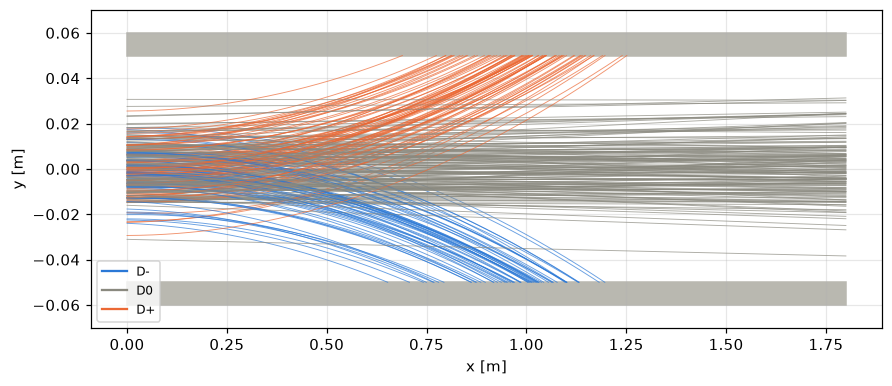

The power on the plates

The power per metre of plate along $x$ : the ions land in a band centred where an ion from the axis reaches the plate, $x = v\sqrt{g / a}$ with $a = eE/m$ (dashed), and as wide as the beam’s width makes it: an ion starting nearer its plate lands earlier. The two plates take the same power, as the beam carries as many D $^-$ as D $^+$ .

edges = np.linspace(0, length, 37)
landing = speed * np.sqrt(gap / (constants.e * voltage / gap / mass))
on_plate = xr.concat(
    [result.wall.subset(result.wall_index == k).along_x(edges) / 1e6 for k in range(2)],
    dim=xr.DataArray(["+y (D+)", "-y (D-)"], dims="plate"),
).assign_attrs(units="MW/m", long_name="power on the plate")
with pp.figure(figsize=(7, 3.4)) as fig:
    for k in range(2):
        on_plate.plasma.plot.lineout(x="x", plate=k, ax=fig[0])
    fig[0].axvline(landing, color="black", ls="--", lw=1)
    fig[0].legend(["+y (D+)", "-y (D-)", "an ion from the axis"], fontsize=8)
print(f"an ion from the axis lands at x = {landing:.2f} m")

an ion from the axis lands at x = 1.00 m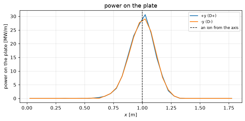

Reionized ions in the stray field

In the duct the gas reionizes a few percent of the neutrals (see the duct tutorial). Without a field they stop where they are born; in the stray field of the tokamak, which grows towards the port, they turn onto the walls. A round duct, 3 m long with a 0.15 m bore, a denser gas than usual to show more of them, and a vertical stray field rising from 10 to 50 mT:

duct_length, bore = 3.0, 0.15
tube = SlantedTube((0, 0, 0), (duct_length, 0, 0), bore, 0.5, (1, 0, 0))
transitions = ChargeStateTransitions({"D2": {("0", "+"): 1.5e-20}})
neutrals = gaussian_beam(30_000, power=16e6, speed=speed, width=0.03, divergence=0.004)
duct = Duct([tube], port=duct_length, transitions=transitions, gas={"D2": 2e18})
reionized = duct.trace(neutrals).reionized
stray = profile_field([0.0, duct_length], [[0, 0], [0, 0], [0.01, 0.05]])
bent = FieldRegion([tube], exit=duct_length, mass=mass, magnetic=stray, step=5e-3)
in_field = bent.trace(reionized)
print(
    f"reionized: {reionized.total_power / 1e3:.0f} kW, "
    f"on the walls: {in_field.wall.total_power / 1e3:.0f} kW, "
    f"through the port: {in_field.exit.total_power / 1e3:.0f} kW"
)

edges = np.linspace(0, duct_length, 31)
compare = xr.concat(
    [reionized.along_x(edges) / 1e3, in_field.wall.along_x(edges) / 1e3],
    dim=xr.DataArray(["where born", "on the wall, in the stray field"], dims="case"),
).assign_attrs(units="kW/m", long_name="reionized power per metre")
with pp.figure(figsize=(7, 3.4)) as fig:
    for k in range(2):
        compare.plasma.plot.lineout(x="x", case=k, ax=fig[0])
    fig[0].legend(["where born", "on the wall, in the stray field"], fontsize=8)

reionized: 1341 kW, on the walls: 825 kW, through the port: 516 kW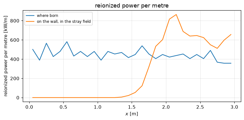

Deposited where they are born, the reionized ions would load the duct evenly along its length. In the stray field they turn towards $-y$ (the force $e\,\mathbf\{v\} \times \mathbf\{B\}$ on a D $^+$ moving along $+x$ in a field along $+z$ ) and land on that side of the bore over the last 1.5 m, where the field is strongest; about 40 % of them, born near the port, leave through it. The load on the duct is thus peaked and one-sided, which the deposit at birth does not show.