Einzel lens optimisation

Download notebook View on GitHubRun when the site was built.

A first design optimisation with beamtracer.optimization: an einzel lens focusing a 30 keV proton beam onto a plane downstream. The optimisation core only calls an evaluation function, here a BeamOptics solve of the lens; any other model can take its place. Differential evolution (SciPy) runs the search, every evaluation is recorded in a JSON-lines file, and a search resumes from its record.

The steps, each checked before the next:

one parameter, the middle voltage, without space charge: the optimiser against a scan and the thin-lens estimate;
three parameters (voltage, gap, aperture) with a limit on the surface field;
space charge on: how far the optimum moves.

import tempfile
from dataclasses import replace
from pathlib import Path

import matplotlib.pyplot as plt
import numpy as np

from beamtracer.optimization import load_record, optimize, scan
from beamtracer.optimization.einzel import EinzelLens

BLUE, ORANGE, AQUA, YELLOW = "#2a78d6", "#eb6834", "#1baf7a", "#eda100"
INK, MUTED, ELECTRODE = "#2b2a26", "#8a897f", "#b9b8b0"
plt.rcParams.update(
    {
        "figure.dpi": 110,
        "axes.edgecolor": MUTED,
        "axes.labelcolor": INK,
        "axes.grid": True,
        "grid.color": "#e4e3dd",
        "grid.linewidth": 0.6,
        "xtick.color": MUTED,
        "ytick.color": MUTED,
        "legend.frameon": False,
        "lines.linewidth": 2,
    }
)
WORKERS = 1  # processes per search
runs = Path(tempfile.mkdtemp())  # the records of this page's searches

The lens

EinzelLens holds the fixed settings and builds the BeamOpticsConfig of a design. Three tubes, 8 mm long and 2 mm thick with half-round ends, sit in a grounded tube of 20 mm radius in cylindrical $(x, r)$ geometry; the outer two are at 0 V, the middle one at the voltage $V$ . A parallel beam of 30 keV protons, 2 mm in radius, starts at $x = 1$ mm, and the objective is its rms size $\sqrt{\langle r^2 \rangle / 2}$ at the target plane $x = 120$ mm. Lost trajectories are a constraint; so is the largest field on the electrode surfaces. A solve on the default 0.5 mm mesh takes a fraction of a second.

lens = EinzelLens()
print(
    f"{lens.energy / 1e3:.0f} keV protons, beam radius {lens.beam_radius * 1e3} mm, "
    f"target at {lens.target * 1e3:.0f} mm, mesh {lens.cell * 1e3} mm"
)
print(
    f"defaults: gap {lens.gap * 1e3} mm, aperture {lens.aperture * 1e3} mm, "
    f"field limit {lens.field_limit / 1e6} MV/m"
)

30 keV protons, beam radius 2.0 mm, target at 120 mm, mesh 0.5 mm
defaults: gap 4.0 mm, aperture 5.0 mm, field limit 5.0 MV/m

Step 1: the voltage

The problem has one parameter. A scan over the voltage and differential evolution share the evaluation and the record: the search takes the designs the scan already evaluated from the record instead of solving them again.

step1 = lens.problem({"voltage": (12e3, 18e3)})
record1 = runs / "step1.jsonl"
voltages = np.linspace(13e3, 17e3, 33)
grid = scan(step1, {"voltage": voltages}, workers=WORKERS, record=record1)
search = optimize(
    step1, seed=1, popsize=8, maxiter=25, tol=1e-6, workers=WORKERS, record=record1
)
thin = lens.thin_lens_voltage()
paraxial = lens.paraxial_voltage()

step = voltages[1] - voltages[0]
print(
    f"scan:      V = {grid.x['voltage']:7.0f} V  spot {grid.fun * 1e6:5.1f} um  ({step:.0f} V steps)"
)
print(
    f"optimiser: V = {search.x['voltage']:7.0f} V  spot {search.fun * 1e6:5.1f} um  "
    f"({search.evaluated} evaluations)"
)
print(
    f"thin lens: V = {thin:7.0f} V  ({thin / search.x['voltage'] - 1:+.1%} of the optimum)"
)
print(f"paraxial:  V = {paraxial:7.0f} V  ({paraxial / search.x['voltage'] - 1:+.1%})")

scan:      V =   14875 V  spot  29.7 um  (125 V steps)
optimiser: V =   14924 V  spot  28.4 um  (121 evaluations)
thin lens: V =   15172 V  (+1.7% of the optimum)
paraxial:  V =   15401 V  (+3.2%)

def spot_and_voltage(evaluations):
    ok = [e for e in evaluations if e.feasible]
    return (
        np.array([e.parameters["voltage"] for e in ok]) / 1e3,
        np.array([e.objectives["spot"] for e in ok]) * 1e6,
    )


fig, axes = plt.subplots(1, 2, figsize=(10, 3.8))
for ax, zoom in zip(axes, (False, True), strict=True):
    v, s = spot_and_voltage(grid.evaluations)
    ax.plot(v, s, color=BLUE, marker="o", ms=4, lw=1.5, label="scan")
    v, s = spot_and_voltage(search.evaluations)
    ax.scatter(
        v, s, s=14, color=ORANGE, alpha=0.6, zorder=3, label="optimiser's evaluations"
    )
    ax.scatter(
        [search.x["voltage"] / 1e3],
        [search.fun * 1e6],
        s=120,
        marker="*",
        color=ORANGE,
        edgecolor="white",
        zorder=4,
        label="optimum",
    )
    ax.axvline(thin / 1e3, color=AQUA, ls="--", lw=1.5, label="thin lens")
    ax.axvline(paraxial / 1e3, color=MUTED, ls=":", lw=1.5, label="paraxial ray")
    ax.set_xlabel("middle voltage [kV]")
    ax.set_ylabel("rms spot at the target [µm]")
    if zoom:
        centre = search.x["voltage"] / 1e3
        ax.set_xlim(centre - 0.6, centre + 0.9)
        ax.set_ylim(0, 160)
        ax.set_title("near the optimum", color=INK, fontsize=10)
    else:
        ax.set_yscale("log")
        ax.set_title("the scan and the search", color=INK, fontsize=10)
axes[1].legend(fontsize=8, loc="upper center")
fig.tight_layout()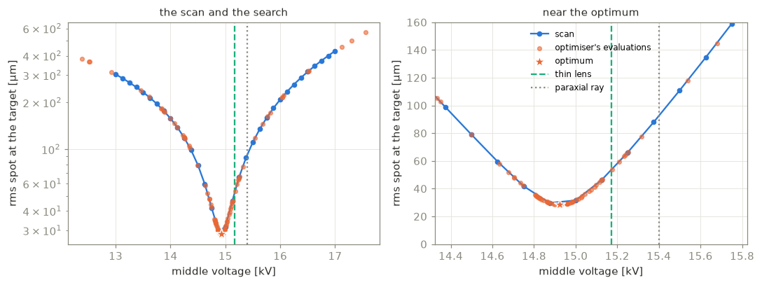

Every evaluation carries the generation of the evolution that asked for it (0 is the initial population), and search.path holds the best design after each generation. SciPy asks for some designs again (it checks the best one between generations); the search answers those from memory, lists each design once and counts the repeats.

path = search.path_to_dataset()
print(
    f"{len(search.path) - 1} generations, {len(search.evaluations)} designs: "
    f"{search.evaluated} solved, {search.reused} from the scan's record, "
    f"{search.repeats} asked for again"
)
fig, ax = plt.subplots(figsize=(7, 3.2))
ax.plot(
    path.generation,
    path.voltage / 1e3,
    color=ORANGE,
    marker="o",
    ms=4,
    label="best of each generation",
)
centre = grid.x["voltage"] / 1e3
ax.axhspan(centre - step / 1e3, centre + step / 1e3, color=BLUE, alpha=0.15)
ax.axhline(centre, color=BLUE, ls="--", lw=1.5, label="scan's minimum ± one step")
ax.set_xlabel("generation")
ax.set_ylabel("middle voltage [kV]")
ax.legend(fontsize=8)
fig.tight_layout()

15 generations, 121 designs: 121 solved, 0 from the scan's record, 25 asked for again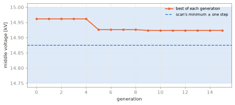

The optimiser lands on the scan’s minimum, within the 125 V step of the scan. The thin-lens estimate, $1/f = \frac{3}{16}\int (\phi'/\phi)^2\,dx$ on the solved axis potential ( $\phi$ the protons’ kinetic energy per charge), and the paraxial ray integrated through the lens both focus at slightly higher voltages: the 2 mm beam fills 40 % of the bore, its outer rays are focused more strongly (spherical aberration), and the smallest rms spot sits below the paraxial focus. The lens is far from weak, $V/U_0 \approx 0.5$ , yet the thin lens and the paraxial ray differ by only 1.5 %.

With a thin beam (0.5 mm) the aberration is gone, and the traced optimum approaches the paraxial focus; moving the target downstream makes the lens weaker, and the thin-lens estimate converges to it.

print("target  V/U0   thin lens  paraxial   traced   thin/traced - 1")
for target in (120e-3, 180e-3, 250e-3):
    weak = replace(
        lens, beam_radius=0.5e-3, num_particles=10, target=target, length=target + 10e-3
    )
    v_thin, v_par = weak.thin_lens_voltage(), weak.paraxial_voltage()
    v = np.linspace(0.97, 1.03, 13) * v_par
    found = scan(
        weak.problem({"voltage": (0.9 * v_par, 1.1 * v_par)}),
        {"voltage": v},
        workers=WORKERS,
    )
    s = np.array([e.objectives["spot"] for e in found.evaluations])
    k = int(np.argmin(s))
    a, b, _ = np.polyfit(v[k - 1 : k + 2], s[k - 1 : k + 2], 2)
    traced = -b / (2 * a)
    print(
        f"{target * 1e3:4.0f} mm  {traced / lens.energy:.2f}  {v_thin:9.0f}  {v_par:8.0f}  {traced:7.0f}  "
        f"{v_thin / traced - 1:+.2%}"
    )

target  V/U0   thin lens  paraxial   traced   thin/traced - 1
 120 mm  0.51      15172     15401    15347  -1.14%
 180 mm  0.41      12299     12418    12366  -0.54%
 250 mm  0.35      10460     10532    10483  -0.22%

The trajectories at the optimum, over the potential:

model = replace(lens, save_trajectories=3).solve(search.x)
potential = model.potential_field.evaluate()
fig, ax = plt.subplots(figsize=(10, 3.6))
mesh = ax.pcolormesh(
    potential.x * 1e3,
    potential.y * 1e3,
    potential.T / 1e3,
    cmap="Blues",
    shading="auto",
)
fig.colorbar(mesh, ax=ax, label="potential [kV]", pad=0.01)
for params in model.config.objects.values():  # a tube is a rectangle and two circles
    for loop in params.build().outlines():
        ax.fill(loop[0] * 1e3, loop[1] * 1e3, color=ELECTRODE, lw=0)
for path in model.trajectories:
    ax.plot(path[:, 0] * 1e3, path[:, 1] * 1e3, color=ORANGE, lw=0.7)
ax.axvline(lens.target * 1e3, color=INK, ls="--", lw=1)
ax.text(lens.target * 1e3 + 1, 10.5, "target", color=INK, fontsize=9)
ax.set_ylim(0, 12)
ax.set_xlabel("x [mm]")
ax.set_ylabel("r [mm]")
ax.set_title(
    f"V = {search.x['voltage'] / 1e3:.2f} kV: every 3rd trajectory",
    color=INK,
    fontsize=10,
)
ax.grid(False)
fig.tight_layout()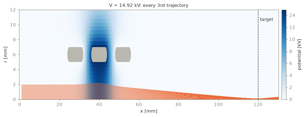

Step 2: voltage, gap and aperture, with a surface-field limit

Three parameters, and the largest field on the electrode surfaces at most 5 kV/mm. The field is that of the solved potential at the nodes next to the electrodes (BeamOptics.surface_fields()); the rounded tube ends keep it finite as the mesh is refined (at a sharp corner it would grow without bound). The searches below are short (about 150 evaluations each, with and without the limit), so their optima are rough.

bounds = {"voltage": (5e3, 25e3), "gap": (1e-3, 12e-3), "aperture": (3e-3, 8e-3)}
settings = dict(seed=1, popsize=4, maxiter=12, tol=1e-4, workers=WORKERS)
free = optimize(lens.problem(bounds), record=runs / "free.jsonl", **settings)
limited = optimize(
    lens.problem(bounds, constraints=("loss", "surface_field")),
    record=runs / "limited.jsonl",
    **settings,
)
for name, result in (("no field limit", free), ("5 kV/mm", limited)):
    x, d = result.x, result.best.diagnostics
    print(
        f"{name:15s} V = {x['voltage'] / 1e3:5.2f} kV  gap {x['gap'] * 1e3:5.2f} mm  "
        f"aperture {x['aperture'] * 1e3:4.2f} mm  spot {result.fun * 1e6:5.1f} um  "
        f"field {d['field'] / 1e6:4.2f} MV/m  ({result.evaluated} evaluations)"
    )

no field limit  V = 14.75 kV  gap  7.95 mm  aperture 3.95 mm  spot  23.0 um  field 5.25 MV/m  (155 evaluations)
5 kV/mm         V = 14.58 kV  gap 10.40 mm  aperture 3.45 mm  spot  57.1 um  field 4.97 MV/m  (156 evaluations)

data = load_record(runs / "limited.jsonl")
fig, axes = plt.subplots(1, 2, figsize=(10, 3.8))
ax = axes[0]
ok = data.ok.values
inside = ok & (data.surface_field.values <= 0)
for mask, color, label in (
    (inside, BLUE, "within the limit"),
    (ok & ~inside, ORANGE, "above the limit"),
):
    ax.scatter(
        data.field[mask] / 1e6,
        data.spot[mask] * 1e6,
        s=10,
        color=color,
        alpha=0.6,
        label=label,
    )
ax.axvline(lens.field_limit / 1e6, color=INK, ls="--", lw=1, label="limit")
for result, marker, label in (
    (free, "D", "optimum, no limit"),
    (limited, "*", "optimum, 5 kV/mm"),
):
    ax.scatter(
        result.best.diagnostics["field"] / 1e6,
        result.fun * 1e6,
        s=180,
        marker=marker,
        color=INK,
        edgecolor="white",
        zorder=4,
        label=label,
    )
ax.set_yscale("log")
ax.set_xlim(1.5, 12)  # a few designs above 12 MV/m are off the plot
ax.set_xlabel("largest surface field [MV/m]")
ax.set_ylabel("rms spot [µm]")
ax.legend(fontsize=8, loc="lower right")
ax = axes[1]
for result, color, label in (
    (free, BLUE, "no field limit"),
    (limited, ORANGE, "5 kV/mm"),
):
    path = result.path_to_dataset()
    ax.plot(
        path.generation, path.spot * 1e6, color=color, marker="o", ms=3, label=label
    )
ax.set_yscale("log")
ax.set_xlabel("generation")
ax.set_ylabel("spot of the best design [µm]")
ax.legend(fontsize=8)
fig.tight_layout()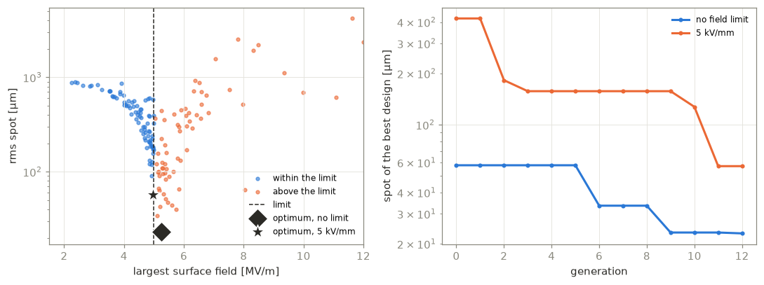

These short searches only start the job. Longer ones (population 30, 60 generations, three seeds, about 1800 evaluations each) settle it. Without a limit they widen the gap and the bore to their bounds (19.8 kV, 12 mm, 8 mm, a 13.9 µm spot): a wider bore keeps the beam nearer the axis (weaker aberrations) and a wider gap makes the potential step gentler, at the price of more voltage, and the field at the rounded tube ends reaches 6.5 MV/m. With the 5 kV/mm limit the constraint is active at the optimum (5.00 MV/m) and the search trades voltage against gap and bore: a narrow bore focuses with less voltage, and the gap settles where widening it further would need more voltage than it saves in field. The three seeds give 14.5–14.6 kV, a 9.6–10.0 mm gap, a 3.46 mm bore and a 36–38 µm spot; the optimum lies in a flat valley along the constraint, so they agree on the field and the bore better than on the gap.

On the 0.5 mm mesh the surface field is underestimated: the same design reads 5.0, 5.2 and 5.6 MV/m on 0.5, 0.25 and 0.125 mm meshes, so the limit given to the search needs a margin of 10–15 % (or a finer mesh for the final design).

Step 3: space charge

With a beam current the Vlasov iteration converges the field and the trajectories together (8–10 iterations, about a second per solve). The space charge defocuses the beam, so the lens needs more voltage, and the smallest spot grows: the optimum moves away from the one without space charge, by about 9 % at 1 mA and 22 % at 3 mA (7 % and 20 % above the thin-lens voltage). The stars are the optimiser’s minima, between the 1 kV steps of the scans; longer searches with three seeds find the same voltages to within 1 V.

fig, ax = plt.subplots(figsize=(7, 3.8))
voltages = np.linspace(13e3, 20e3, 8)
optima = {0.0: search}
for current, color in ((0.0, BLUE), (1e-3, ORANGE), (3e-3, AQUA)):
    charged = replace(lens, current=current)
    problem = charged.problem({"voltage": (12e3, 21e3)})
    record = runs / f"space_charge_{current * 1e3:.0f}mA.jsonl"
    swept = scan(problem, {"voltage": voltages}, workers=WORKERS, record=record)
    if current > 0.0:
        optima[current] = optimize(
            problem,
            seed=1,
            popsize=4,
            maxiter=6,
            tol=1e-5,
            workers=WORKERS,
            record=record,
        )
    found = optima[current]
    v, s = spot_and_voltage(swept.evaluations)
    ax.plot(
        v, s, color=color, marker="o", ms=3, lw=1.5, label=f"{current * 1e3:.0f} mA"
    )
    ax.scatter(
        found.x["voltage"] / 1e3,
        found.fun * 1e6,
        s=140,
        marker="*",
        color=color,
        edgecolor="white",
        zorder=4,
    )
ax.scatter([], [], s=140, marker="*", color=MUTED, label="optimiser")
ax.axvline(
    thin / 1e3, color=MUTED, ls="--", lw=1.5, label="thin lens (no space charge)"
)
ax.set_yscale("log")
ax.set_xlabel("middle voltage [kV]")
ax.set_ylabel("rms spot at the target [µm]")
ax.legend(fontsize=8, title="beam current", title_fontsize=8)
fig.tight_layout()
for current, found in optima.items():
    shift = found.x["voltage"] / optima[0.0].x["voltage"] - 1
    print(
        f"{current * 1e3:.0f} mA: V = {found.x['voltage']:6.0f} V ({shift:+.1%}), "
        f"spot {found.fun * 1e6:5.1f} um, "
        f"{found.best.diagnostics['iterations']} Vlasov iterations"
    )

0 mA: V =  14924 V (+0.0%), spot  28.4 um, 1 Vlasov iterations
1 mA: V =  16260 V (+9.0%), spot  58.6 um, 8 Vlasov iterations
3 mA: V =  17946 V (+20.3%), spot 167.8 um, 10 Vlasov iterations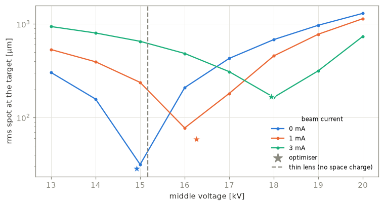

The record

Every evaluation of a search is a line of its record, with the parameters, objectives, constraints, the converged flag, the wall time, diagnostics and the generation that asked for it (-1 for the scan’s designs). load_record reads it as an xarray Dataset (.to_dataframe() for pandas), and a search given the same record and seed continues from it without solving the recorded designs again.

data = load_record(record1)
print(
    data[["voltage", "spot", "loss", "converged", "generation"]].to_dataframe().tail()
)
again = optimize(step1, seed=1, popsize=8, maxiter=25, tol=1e-6, record=record1)
print(f"rerun: {again.evaluated} new evaluations, {again.reused} from the record")

                 voltage      spot  loss  converged  generation
evaluation
149         14923.175701  0.000028   0.0       True          15
150         14923.911827  0.000028   0.0       True          15
151         14923.778181  0.000028   0.0       True          15
152         14923.374953  0.000028   0.0       True          15
153         14923.603731  0.000028   0.0       True          15
rerun: 0 new evaluations, 121 from the record