Duct

Download notebook View on GitHubRun when the site was built.

Beyond the accelerator and the neutralizer no field acts on the neutrals: they fly on straight lines to the port. beamtracer.beamline.Duct intersects each line with the duct walls, given as simgeometry shapes, without a mesh, and samples where the duct gas reionizes a neutral (an exponential free path). A reionized neutral is deposited where it is born, a bound on where its power goes until the stray field that bends it is added.

The beam here is a round Gaussian beam of 1 MeV deuterium atoms, as Markers in 3D; the duct a rectangular channel of four plates. The cross section is a placeholder: plasmacoll holds no beam stripping data, so it is an input.

import matplotlib.patches as patches
import numpy as np
import plasma_plots as pp
import xarray as xr
from plasmacoll import ChargeStateTransitions
from scipy import constants
from simgeometry import Cuboid, SlantedTube

from beamtracer.beamline import Duct, gaussian_beam

BLUE, ORANGE, AQUA, MUTED = "#2a78d6", "#eb6834", "#1baf7a", "#8a897f"

energy = 1e6 * constants.e  # 1 MeV
mass = 2.014 * constants.atomic_mass
speed = np.sqrt(2 * energy / mass)
beam = gaussian_beam(
    200_000, power=16e6, speed=speed, width=0.06, divergence=0.007, seed=1
)

length, half_y, half_z, wall = 3.0, 0.15, 0.3, 0.05
walls = [
    Cuboid(
        (length / 2, s * (half_y + wall / 2), 0), (length, wall, 2 * (half_z + wall))
    )
    for s in (1, -1)
] + [
    Cuboid((length / 2, 0, s * (half_z + wall / 2)), (length, 2 * half_y, wall))
    for s in (1, -1)
]
transitions = ChargeStateTransitions({"D2": {("0", "+"): 1.5e-20}})
duct = Duct(walls, port=length, transitions=transitions, gas={"D2": 1e18})
result = duct.trace(beam)
result.summary()

Where the beam goes

A side view: a few hundred of the lines, coloured by where they end, and the two plates at $y = \pm 0.15$ m. Most of the beam reaches the port; its tails scrape the plates over the last metre, where the beam has spread; a few percent are reionized anywhere along the duct.

def lines(markers, start, count):
    take = np.arange(min(count, len(markers)))
    return start.position[:, take], markers.position[:, take]


rng = np.random.default_rng(0)
order = rng.permutation(len(beam))
first = beam.subset(order)
traced = duct.trace(first.subset(slice(0, 400)))
start = first.subset(slice(0, 400))
fates = {
    "port": (traced.port, BLUE),
    "wall": (traced.wall, ORANGE),
    "reionized": (traced.reionized, AQUA),
}
with pp.figure(figsize=(8, 3.2)) as fig:
    ax = fig[0]
    for s in (1, -1):
        y0 = half_y if s > 0 else -half_y - wall
        ax.add_patch(patches.Rectangle((0, y0), length, wall, color=MUTED, alpha=0.4))
    # the start of each fate's lines, matched through their velocity
    for label, (markers, color) in fates.items():
        if len(markers) == 0:
            continue
        x1, y1 = markers.position[0], markers.position[1]
        slope = markers.velocity[1] / markers.velocity[0]
        y0 = y1 - slope * x1
        ax.plot([np.zeros_like(x1), x1], [y0, y1], color=color, lw=0.5, alpha=0.6)
        ax.plot([], [], color=color, label=f"{label} ({len(markers)})")
    ax.set_xlabel("x [m]")
    ax.set_ylabel("y [m]")
    ax.set_ylim(-0.25, 0.25)
    ax.legend(loc="lower left", fontsize=8)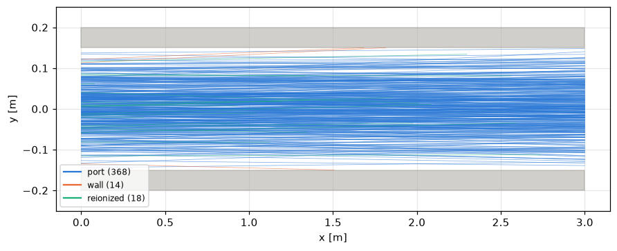

The footprint at the port

The power density of the neutrals in the port plane: the round beam, clipped at $y = \pm 0.15$ m by the narrow plates; the wide ones ( $z = \pm 0.3$ m) take almost nothing.

footprint = result.port.footprint(bins=60, extent=(-0.3, 0.3, -0.3, 0.3))
(footprint / 1e6).assign_attrs(
    units="MW/m²", long_name="power density"
).plasma.plot.slice(
    x="y", y="z", equal_aspect=True, colorbar_label="power density [MW/m²]"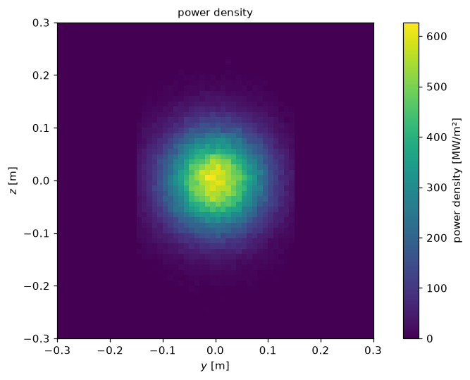
)

The power on the walls

The power per metre of duct on the plates, against $x$ . The peak at the entrance is the beam’s tails outside the bore there (beyond $y = \pm 0.15$ m, 2.5 widths out): they start in the plates and stop on their front faces. Along the duct the power grows towards the port, where the beam is widest.

edges = np.linspace(0, length, 31)
on_walls = (result.wall.along_x(edges) / 1e3).assign_attrs(
    units="kW/m", long_name="power on the walls"
)
on_walls.plasma.plot.lineout(x="x")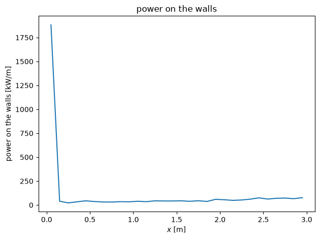

Transmission against the closed form

The lines are straight and the duct is convex, so a line inside at both ends is inside all the way: the transmission is the share of the beam inside the bore at the port. For a round bore of radius $a$ that is $1 - \exp(-a^2 / 2\sigma^2)$ , with $\sigma^2 = w^2 + (L\theta)^2$ the beam’s width at the port, as long as the beam starts inside the bore. Without gas, a narrow beam (5 mm, 20 mrad) through circular ducts of a range of bores (a tube cut square at its end):

narrow = gaussian_beam(
    200_000, power=16e6, speed=speed, width=0.005, divergence=0.02, seed=2
)
sigma = np.hypot(0.005, length * 0.02)
bores = np.linspace(0.02, 0.15, 9)
measured = []
for bore in bores:
    tube = SlantedTube((0, 0, 0), (length, 0, 0), bore, 1.0, (1, 0, 0))
    measured.append(Duct([tube], port=length).trace(narrow).transmission)
transmission = xr.DataArray(
    measured, dims="bore", coords={"bore": bores}, name="transmission"
)
transmission.plasma.plot.against_theory(
    lambda a: 1 - np.exp(-(a**2) / (2 * sigma**2)),
    xlabel="bore radius [m]",
    ylabel="transmission",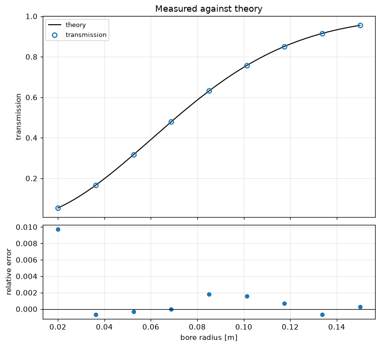
)

The relative error stays at the sampling noise of 200 000 markers. The square duct is checked the same way in the tests, against $\mathrm{erf}(a / \sqrt{2}\sigma)^2$ , the formula of freeofcharge’s duct_transmission.

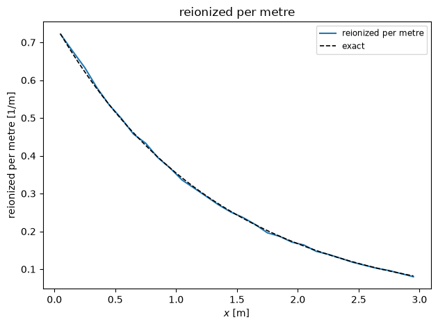
Reionization along the duct

Where the neutrals are reionized, per metre: with a uniform gas the rate falls as $n\sigma \exp(-n\sigma x)$ of the power entering. A denser gas than above (5e19 m⁻³) makes the fall visible over the duct:

dense = Duct([], port=length, transitions=transitions, gas={"D2": 5e19})
reionized = dense.trace(beam).reionized
k = 5e19 * 1.5e-20
per_length = (reionized.along_x(edges) / beam.total_power).assign_attrs(
    units="1/m", long_name="reionized per metre"
)
per_length.plasma.plot.lineout(x="x", reference=lambda x: k * np.exp(-k * x))
print(
    f"reionized: {reionized.total_power / beam.total_power:.1%}, "
    f"expected {1 - np.exp(-k * length):.1%}"
)

reionized: 89.4%, expected 89.5%