Grid

Download notebookView on GitHubRun when the site was built.

BeamOptics traces one beamlet, in 2D: a round aperture in cylindrical $(x, r)$ geometry, where each trajectory stands for a ring, or a slit in planar geometry. The beamline needs the whole beam in 3D. beamlet_markers turns the beamlet’s crossings of its exit plane into 3D markers (each ring copied at random azimuths), and ApertureGrid copies them to every aperture of the grid, aimed by the grid’s curvature and by steering.

The beamlet is the coarse H$^-$ beamlet of the tutorial on its optimisation, at 8 kV extraction and 20 kV in total.

import numpy as np
import plasma_plots as pp
import xarray as xr

from beamtracer.beamline import ApertureGrid, beamlet_markers, gaussian_beam
from beamtracer.optimization.beamlet import COARSE, NegativeIonBeamlet

case = NegativeIonBeamlet(**COARSE)
model = case.solve({"extraction_voltage": 8e3, "eg_radius": 3e-3, "gap": 4e-3})
hits = model.plane(case.exit_plane)
h_minus = model.species_names.index("H-")
beamlet = beamlet_markers(
    hits,
    mass=model.species_mass[h_minus],
    cylindrical=True,
    species=h_minus,
    copies=200,
    charge=1.0,
)
moments = model.beam_moments(case.exit_plane, "H-")
slope = beamlet.velocity[1] / beamlet.velocity[0]
print(
    f"{len(beamlet)} markers, {beamlet.total_power:.1f} W, "
    f"rms angle (BeamOptics) {moments.rms_angle * 1e3:.1f} mrad, "
    f"(markers, in y) {np.sqrt(np.average(slope**2, weights=beamlet.power)) * 1e3:.1f} mrad"
)

20000 markers, 268.9 W, rms angle (BeamOptics) 27.6 mrad, (markers, in y) 27.3 mrad

The beamlet at its exit plane and 0.5 m further on: the rings of the 2D trace spread round the axis. The power-weighted rms angle of the markers in one plane ($y$) is the rms angle of the traced beamlet, whose moments project the rings on one plane the same way (up to the sampling of the azimuths).

with pp.figure(1, 2, figsize=(9, 3.8)) as fig:
    for k, x in enumerate((case.exit_plane, case.exit_plane + 0.5)):
        half = 4e-3 if k == 0 else 0.03
        footprint = beamlet.drift_to(x).footprint(
            bins=50, extent=(-half, half, -half, half)
        )
        footprint.plasma.plot.slice(
            x="y",
            y="z",
            equal_aspect=True,
            ax=fig[k],
            title=f"x = {x:.2f} m",
            colorbar_label="power density [W/m²]",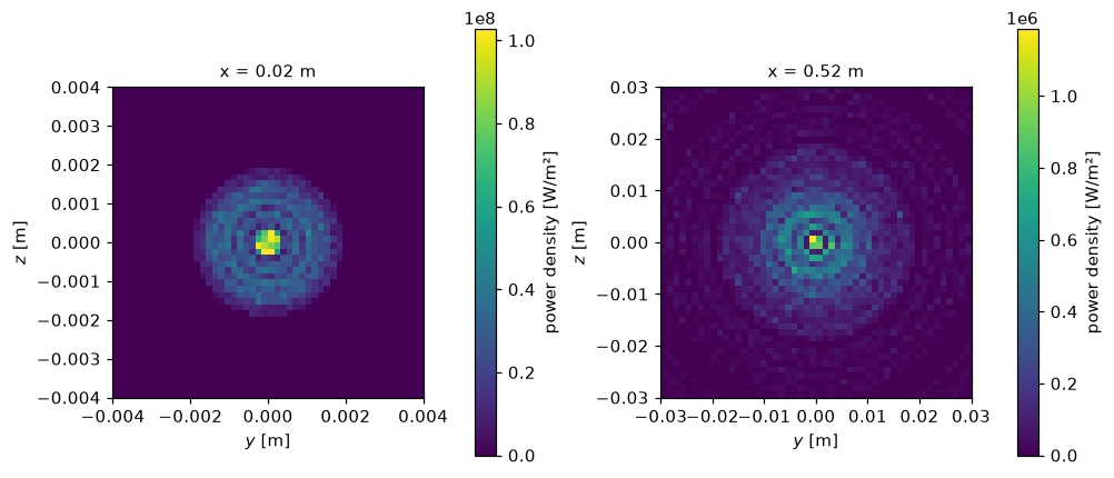
        )

A group of apertures

One beamlet group of ITER’s grid has 5 by 16 apertures, 20 mm apart in $y$ and 22 mm in $z$. Flat, every beamlet keeps its own axis and the beam is the group’s size plus a beamlet’s; curved, the grid aims the beamlets at a point on the axis, where the beam shrinks to one beamlet.

The coarse beamlet above diverges by 27 mrad (the tutorial’s optimum is not much better): over 7 m it spreads far more than the group is wide, and the aim would not show. So the group is made of a Gaussian beamlet of 5 mrad, ITER’s requirement, here; any Markers serve as the beamlet. The group is curved to 7 m in both directions, and the footprints are drawn at 0, 3.5 and 7 m.

narrow = gaussian_beam(
    4000,
    power=beamlet.total_power,
    speed=np.mean(beamlet.velocity[0]),
    width=2e-3,
    divergence=5e-3,
    state="-",
)
flat = ApertureGrid.regular(16, 5, (0.020, 0.022))
curved = ApertureGrid.regular(16, 5, (0.020, 0.022), focal_length=(7.0, 7.0))
beams = {"flat": flat.markers(narrow), "curved to 7 m": curved.markers(narrow)}
distances = (0.0, 3.5, 7.0)
with pp.figure(2, 3, figsize=(11, 8)) as fig:
    for row, (label, beam) in enumerate(beams.items()):
        for col, x in enumerate(distances):
            beam.drift_to(x).footprint(
                bins=150, extent=(-0.3, 0.3, -0.3, 0.3)
            ).plasma.plot.slice(
                x="y",
                y="z",
                equal_aspect=True,
                ax=fig[3 * row + col],
                title=f"{label}, x = {x} m",
                colorbar_label="W/m²",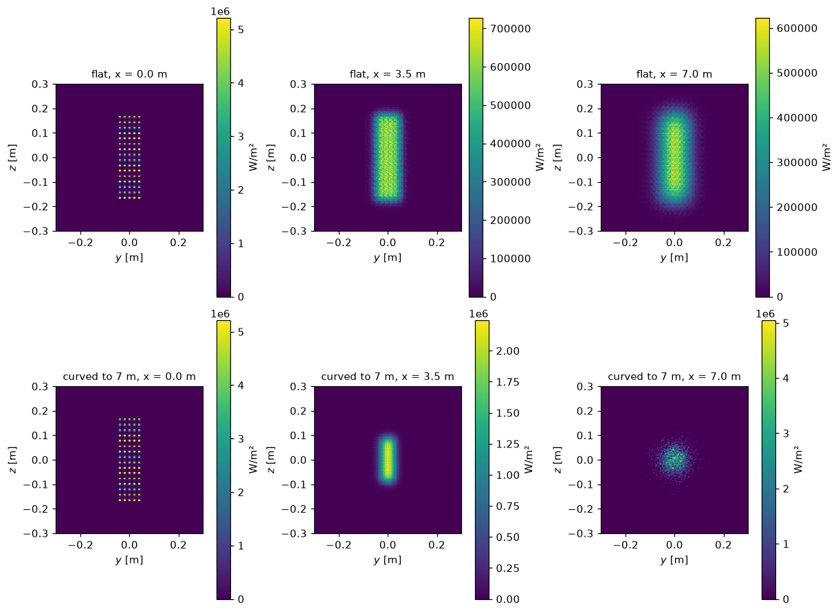
            )

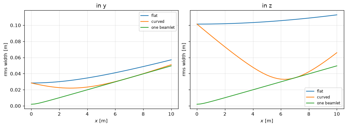
The width of the beam along $x$

The rms width (power-weighted, about the axis) of the whole beam in $y$ and $z$ against the distance. Flat, it grows from the group’s size; curved, it meets that of one beamlet at the focus, where every beamlet’s axis crosses the axis, and follows it beyond. Its minimum lies before the focus, as the beamlets spread while they converge.

xs = np.linspace(0.0, 10.0, 41)


def widths(beam):
    w = np.array(
        [
            np.sqrt(
                np.average(
                    beam.drift_to(x).position[1:] ** 2, axis=1, weights=beam.power
                )
            )
            for x in xs
        ]
    )
    return xr.DataArray(
        w.T,
        dims=("direction", "x"),
        coords={"direction": ["y", "z"], "x": ("x", xs, {"units": "m"})},
        name="width",
        attrs={"units": "m", "long_name": "rms width"},
    )


single = widths(narrow)
with pp.figure(1, 2, figsize=(10, 3.6), sharey=True) as fig:
    for k, direction in enumerate(("y", "z")):
        for beam in beams.values():
            widths(beam).plasma.plot.lineout(x="x", direction=k, ax=fig[k])
        single.plasma.plot.lineout(x="x", direction=k, ax=fig[k])
        fig[k].legend(["flat", "curved", "one beamlet"], fontsize=8)
        fig[k].set_title(f"in {direction}")