7. Notebook magics#
Install for this tutorial:
pip install "scope-profiler[notebook,pproc,line-profiler]".
scope-profiler ships eleven IPython magics that wrap the same
ProfileManager.session()/region() API the other tutorials use by
hand: %%scope, %scope_timeit, %%scope_line, %%scope_recursive,
%%scope_agg, %scope_load, %scope_df, %scope_last,
%scope_compare, %scope_export, and %scope_reset. They are meant
for the “how long is this cell/line taking, and did my change help” loop
you run dozens of times while developing in a notebook, without writing
the session boilerplate out each time.
The combined install above adds IPython, the plotting/DataFrame
dependencies, and line_profiler. The equivalent explicit groups are:
pip install "scope-profiler[notebook,pproc,line-profiler]"
Nothing here writes an HDF5 file — every magic below runs with
deactivate_file_output=True, so results live only in the kernel’s
memory for the duration of this session. See
Jupyter/IPython magics for the full reference.
%load_ext scope_profiler.ipython_magics

import time

from scope_profiler import ProfileManager
A toy workload#
Two versions of the same computation, one deliberately slower than the
other, so there is something worth comparing below. time.sleep stands
in for real work, as in the other tutorials, so the timings are stable
regardless of the machine running this notebook.
def naive_sum_of_squares(n):
    total = 0
    for i in range(n):
        time.sleep(0.0001)  # pretend each term is expensive to compute
        total += i * i
    return total


def fast_sum_of_squares(n):
    # closed form: 0^2 + 1^2 + ... + (n-1)^2
    time.sleep(0.001)  # a little fixed overhead, no per-term cost
    return (n - 1) * n * (2 * n - 1) // 6
%%scope — profile a cell#
%%scope name runs the cell inside a profiling region called name
(default "cell") and prints the summary table right after. The result
is kept in memory under that name for %scope_last/%scope_compare to
refer back to.
%%scope naive
result_naive = naive_sum_of_squares(50)
result_naive
40425

%%scope 'naive'
  ╭──────────────────────────────────────────────────────╮
  │ region                    % session      total [s]   │
  ├──────────────────────────────────────────────────────┤
  │ scope_profiler.session    100.00%        0.009990    │
  │ └─ (own)                     1.88%          0.000188 │
  │ └─ naive                     98.12%         0.009802 │
  ╰──────────────────────────────────────────────────────╯
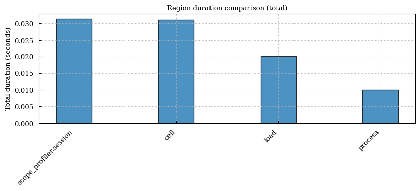
Nested regions work exactly as they do in a script — %%scope only adds
the outer region and the in-memory session. Add -p/--plot to also
show a duration bar chart of everything the cell recorded, or -q to
skip the printed table (the run is still recorded).
%%scope -p
with ProfileManager.region("load"):
    time.sleep(0.02)

with ProfileManager.region("process"):
    time.sleep(0.01)
%%scope 'cell'
  ╭────────────────────────────────────────────────────────╮
  │ region                    % session      total [s]     │
  ├────────────────────────────────────────────────────────┤
  │ scope_profiler.session    100.00%        0.031370      │
  │ └─ (own)                     0.65%          0.000203   │
  │ └─ cell                      99.35%         0.031167   │
  │ │ └─ (own)                     3.23%          0.001012 │
  │ │ └─ load                      64.01%         0.020081 │
  │ │ └─ process                   32.11%         0.010075 │
  ╰────────────────────────────────────────────────────────╯
%scope_timeit — time a statement#
%scope_timeit answers the same question as the built-in %timeit, but
through scope-profiler’s own region timer and table, so its output is
directly comparable to %%scope/%scope_compare.
%scope_timeit -n 5 fast_sum_of_squares(50)
%scope_timeit 'fast_sum_of_squares(50)' (5 runs)
  ╭──────────────────────────────────────────────────────────────────────────────────────────╮
  │ region                    n      total [s]      avg/call [s]      min [s]      max [s]   │
  ├──────────────────────────────────────────────────────────────────────────────────────────┤
  │ scope_profiler.session    1      0.005760       5.760e-03         0.006        0.006     │
  │ └─ (own)                            0.000203       2.028e-04                             │
  │ └─ timeit                 5         0.005557       1.111e-03      0.001        0.001     │
  ╰──────────────────────────────────────────────────────────────────────────────────────────╯
%%scope_recursive — profile a cell with nothing instrumented#
Everything so far needed you to say what to measure.
%%scope_recursive does not: it records every Python call the cell
makes as its own region, so it answers “where did the time go?” before
you know what to instrument. This is recursive_profile=True — the same
thing scope-profiler run does to a script.
%%scope_recursive
def step(values):
    return [value * 2 for value in values]


def simulate(num_steps):
    values = list(range(2_000))
    for _ in range(num_steps):
        values = step(values)
        time.sleep(0.001)
    return values


final = simulate(10)
%%scope_recursive 'cell'
  ╭─────────────────────────────────────────────────────────────────────────────────╮
  │ region                                  % session           total [s]           │
  ├─────────────────────────────────────────────────────────────────────────────────┤
  │ scope_profiler.session                  100.00%             0.012270            │
  │ └─ (own)                                   1.10%               0.000134         │
  │ └─ cell                                    98.90%              0.012135         │
  │ │ └─ (own)                                   0.27%               0.000033       │
  │ │ └─ __main__.<module>                       98.64%              0.012102       │
  │ │ │ └─ (own)                                   0.12%               0.000015     │
  │ │ │ └─ __main__.simulate                       98.51%              0.012087     │
  │ │ │ │ └─ (own)                                   89.95%              0.011037   │
  │ │ │ │ └─ __main__.step (10x)                     8.56%               0.001050   │
  │ │ │ │ │ └─ (own)                                   0.71%               0.000087 │
  │ │ │ │ │ └─ __main__.<listcomp> (10x)               7.85%               0.000964 │
  ╰─────────────────────────────────────────────────────────────────────────────────╯
The table is sorted by total time and nests by call depth, so simulate
and step show up on their own without a single decorator. Use this
first, then reach for %%scope/%%scope_line on whatever it points at.
Two things to keep in mind: library internals called from the cell are
traced too (noisy, and each traced call costs overhead — keep such cells
small, and filter with --include), and the cell runs via exec, so a
trailing expression is not echoed as Out[n].
%%scope_agg — aggregation mode for very hot regions#
A region entered a million times would store a million timestamps. With
aggregation_mode=True each region keeps only its count, total, min/max
and exclusive time — bounded memory, and cheap enough to leave in a hot
loop.
%%scope_agg hot
for _ in range(50_000):
    with ProfileManager.region("tick"):
        pass
%%scope_agg 'hot'
  ╭──────────────────────────────────────────────────────╮
  │ region                    % session      total [s]   │
  ├──────────────────────────────────────────────────────┤
  │ scope_profiler.session    100.00%        0.108624    │
  │ hot                       99.89%         0.108507    │
  │ tick (50kx)               21.59%         0.023455    │
  ╰──────────────────────────────────────────────────────╯
The trade-off: there is no per-call timeline, so Gantt charts and
%scope_df --events have nothing to show for this run. Summaries and
comparisons work as usual.
%scope_last — reprint a previous run#
Reprints a recorded run’s table without re-running anything — handy
after scrolling past a result, or to re-render it with a different
--include. With no name, it reprints the most recently recorded run:
%scope_last
'hot' (last)
  ╭──────────────────────────────────────────────────────╮
  │ region                    % session      total [s]   │
  ├──────────────────────────────────────────────────────┤
  │ scope_profiler.session    100.00%        0.108624    │
  │ hot                       99.89%         0.108507    │
  │ tick (50kx)               21.59%         0.023455    │
  ╰──────────────────────────────────────────────────────╯
Or name one explicitly:
%scope_last naive
'naive' (last)
  ╭──────────────────────────────────────────────────────╮
  │ region                    % session      total [s]   │
  ├──────────────────────────────────────────────────────┤
  │ scope_profiler.session    100.00%        0.009990    │
  │ └─ (own)                     1.88%          0.000188 │
  │ └─ naive                     98.12%         0.009802 │
  ╰──────────────────────────────────────────────────────╯
%scope_compare — compare two runs#
Record the optimized version under its own name, then compare it against
the naive one region-by-region — the same table scope-profiler diff
prints for two HDF5 files, here for two in-notebook runs.
%%scope optimized
result_optimized = fast_sum_of_squares(50)
assert result_optimized == result_naive
%%scope 'optimized'
  ╭──────────────────────────────────────────────────────╮
  │ region                    % session      total [s]   │
  ├──────────────────────────────────────────────────────┤
  │ scope_profiler.session    100.00%        0.001587    │
  │ └─ (own)                     6.83%          0.000108 │
  │ └─ optimized                 93.17%         0.001479 │
  ╰──────────────────────────────────────────────────────╯
%scope_compare naive optimized
'naive' -> 'optimized'
  ╭────────────────────────┬─────────────────┬─────────────────┬─────────────┬─────────────╮
  │ region                 │ total [s] (a)   │ total [s] (b)   │ delta       │ delta [%]   │
  ├────────────────────────┼─────────────────┼─────────────────┼─────────────┼─────────────┤
  │ naive                  │ 0.00980201      │ -               │ -0.00980201 │ -100%       │
  │ scope_profiler.session │ 0.00998978      │ 0.0015872       │ -0.00840259 │ -84.11%     │
  │ optimized              │ -               │ 0.00147885      │ +0.00147885 │ -           │
  ╰────────────────────────┴─────────────────┴─────────────────┴─────────────┴─────────────╯

  Only in a: naive
  Only in b: optimized
Regions are matched by name, so naive and optimized - named after
their own %%scope cell - each show up as “only in a”/“only in b”:
there is nothing on the other side to diff them against.
scope_profiler.session, the outer region every run has, is present
in both, and its row is the real before/after number. To get a
per-region diff instead of just the session total, give the part you
want compared the same name in both cells, e.g. wrap it in
ProfileManager.region("compute") inside each %%scope cell.
With no arguments, %scope_compare compares the two most recently
recorded runs, so plain %scope_compare would have worked here too.
Pass --metric (total, avg, min, max, p50, p95, p99,
imbalance, or calls) or --sort (delta, pct, name) to change
what is compared or how rows are ordered.
%scope_compare naive optimized --metric avg --sort name
'naive' -> 'optimized'
  ╭────────────────────────┬───────────────┬───────────────┬─────────────┬─────────────╮
  │ region                 │ avg [s] (a)   │ avg [s] (b)   │ delta       │ delta [%]   │
  ├────────────────────────┼───────────────┼───────────────┼─────────────┼─────────────┤
  │ naive                  │ 0.00980201    │ -             │ -0.00980201 │ -100%       │
  │ optimized              │ -             │ 0.00147885    │ +0.00147885 │ -           │
  │ scope_profiler.session │ 0.00998978    │ 0.0015872     │ -0.00840259 │ -84.11%     │
  ╰────────────────────────┴───────────────┴───────────────┴─────────────┴─────────────╯

  Only in a: naive
  Only in b: optimized
%%scope_line — line-by-line profiling for a cell#
Wall-clock totals tell you that naive_sum_of_squares is slow; line
profiling tells you which line. %%scope_line runs the cell with
use_line_profiler=True and prints per-line hit counts and time for
whatever the cell hands to line_profiler - needs the line-profiler
extra. Prefer decorating the function you care about with
@ProfileManager.profile, as below: it registers cleanly regardless of
where it’s called from.
%%scope_line
@ProfileManager.profile("naive_line")
def naive_sum_of_squares_traced(n):
    total = 0
    for i in range(n):
        time.sleep(0.0001)
        total += i * i
    return total


naive_sum_of_squares_traced(20)
2470

%%scope_line 'cell'
  ╭──────────────────────────────────────────────────────╮
  │ region                    % session      total [s]   │
  ├──────────────────────────────────────────────────────┤
  │ scope_profiler.session    100.00%        0.006822    │
  │ └─ (own)                     50.03%         0.003413 │
  │ └─ naive_line                49.97%         0.003409 │
  ╰──────────────────────────────────────────────────────╯

Timer unit: 1e-09 s

Total time: 0.00338904 s
File: /tmp/ipykernel_4699/189735869.py
Function: naive_sum_of_squares_traced at line 1

Line #      Hits         Time  Per Hit   % Time  Line Contents
==============================================================
     1                                           @ProfileManager.profile("naive_line")
     2                                           def naive_sum_of_squares_traced(n):
     3         1        381.0    381.0      0.0      total = 0
     4        21       4680.0    222.9      0.1      for i in range(n):
     5        20    3374869.0 168743.5     99.6          time.sleep(0.0001)
     6        20       8925.0    446.2      0.3          total += i * i
     7         1        181.0    181.0      0.0      return total
The time.sleep line dominates the table, as expected - in a real
workload this is exactly how you’d spot the line actually worth
optimizing.
%scope_export — save a run to a file#
A recorded run doesn’t have to stay in the notebook. Export it to a
.prof file for snakeviz/pstats, or to speedscope JSON, via
export_prof/export_speedscope - the same functions
scope-profiler export uses on an HDF5 file, here applied directly to
the in-memory result.
import tempfile
from pathlib import Path

export_dir = Path(tempfile.mkdtemp(prefix="scope-profiler-tutorial-"))
%scope_export -n optimized {export_dir}/optimized.prof
%scope_export -n optimized {export_dir}/optimized.speedscope.json
sorted(p.name for p in export_dir.iterdir())
wrote /tmp/scope-profiler-tutorial-l0_ikq7x/optimized_rank0.prof
wrote /tmp/scope-profiler-tutorial-l0_ikq7x/optimized.speedscope.json

['optimized.speedscope.json', 'optimized_rank0.prof']
%scope_load — compare against a run from outside the notebook#
Profiling data from an MPI job or a scope-profiler run is just an HDF5
file. %scope_load reads one (via read_h5) into the same name
registry the cell magics use, so a cluster run becomes directly
comparable with what you just measured here. Let’s write one out to
stand in for that file.
cluster_file = export_dir / "cluster_run.h5"
with ProfileManager.session(file_path=str(cluster_file), verbose=False):
    with ProfileManager.region("optimized"):
        fast_sum_of_squares(50)

%scope_load {cluster_file}
%scope_load /tmp/scope-profiler-tutorial-l0_ikq7x/cluster_run.h5 as 'cluster_run'
  ╭──────────────────────────────────────────────────────╮
  │ region                    % session      total [s]   │
  ├──────────────────────────────────────────────────────┤
  │ scope_profiler.session    100.00%        0.001149    │
  │ └─ (own)                     6.54%          0.000075 │
  │ └─ optimized                 93.46%         0.001073 │
  ╰──────────────────────────────────────────────────────╯
%scope_compare cluster_run optimized
'cluster_run' -> 'optimized'
  ╭────────────────────────┬─────────────────┬─────────────────┬──────────────┬─────────────╮
  │ region                 │ total [s] (a)   │ total [s] (b)   │ delta        │ delta [%]   │
  ├────────────────────────┼─────────────────┼─────────────────┼──────────────┼─────────────┤
  │ scope_profiler.session │ 0.00114856      │ 0.0015872       │ +0.000438635 │ +38.19%     │
  │ optimized              │ 0.00107348      │ 0.00147885      │ +0.000405363 │ +37.76%     │
  ╰────────────────────────┴─────────────────┴─────────────────┴──────────────┴─────────────╯
%scope_df — the run as a pandas DataFrame#
For anything the printed table doesn’t cover, take the DataFrame: it is the magic’s return value, so it renders on its own and can be assigned and analysed further — everything tutorial 2 does with a file, on the run you just measured.
df = %scope_df -n optimized
df[["name", "num_calls", "total_duration", "average_duration"]]
name |
num_calls |
total_duration |
average_duration |
|
|---|---|---|---|---|
0 |
scope_profiler.session |
1 |
0.001587 |
0.001587 |
1 |
optimized |
1 |
0.001479 |
0.001479 |
%scope_df --events -n optimized
name |
rank |
call_index |
start |
end |
duration |
|
|---|---|---|---|---|---|---|
0 |
scope_profiler.session |
0 |
0 |
0.001483 |
0.003070 |
0.001587 |
1 |
optimized |
0 |
0 |
0.001588 |
0.003067 |
0.001479 |
%scope_reset — drop recorded runs#
Recorded runs accumulate in memory for the life of the kernel. Clear one by name, then clear everything else that is left:
%scope_reset naive
%scope_reset
cleared recorded run 'naive'
cleared all recorded scope-profiler runs
Where to go next#
These magics are a thin layer over ProfileManager and
ProfilingResults — everything from 2. Post-processing profiling data and
3. Visualizing results (custom filtering, DataFrames, Gantt/flame
charts) still works on the ProfilingResults objects they record; reach
into get_ipython().magics_manager.registry["ScopeMagics"]._runs if you
want one back as a Python object instead of a printed table.