Plotting with the CLI#
Install for this page:
pip install "scope-profiler[pproc]", including the optional interactive PyVis call-graph backend.
scope-profiler plot turns one or more profiling_data.h5 files into
charts and an aggregate statistics JSON. scope-profiler export writes
the same plot data and external viewer formats without rendering images.
Together they cover the same ground as the plotting functions described
in HDF5 output & post-processing from Python, without writing any code. For
text/JSON summaries instead of figures — including LIKWID hardware
counters — see scope-profiler inspect in CLI reference.
This page walks through the command with a concrete example. For the complete list of flags, see CLI reference.
The example run#
Every figure below comes from the same mock solver: a setup phase
followed by three timesteps, each containing assemble, solve and
halo_exchange, with io on every second step. It was run at 1, 2 and
4 MPI ranks, producing run_1.h5, run_2.h5 and run_4.h5:
with ProfileManager.region("setup"):
    ...

for step in range(3):
    with ProfileManager.region("timestep"):
        with ProfileManager.region("assemble"):
            ...
        with ProfileManager.region("solve"):
            ...
        with ProfileManager.region("halo_exchange"):
            ...
        if step % 2 == 1:
            with ProfileManager.region("io"):
                ...
The complete script, including the commands used to render every figure
on this page, is examples/generate_cli_docs_figures.py.
Basic usage#
Choose a plot preset and give it an output directory:
scope-profiler plot default run_2.h5 -o figures
Plotting Gantt chart for ranks: [0]
Plotting duration comparison (total) for files: run_2
Outputs saved to:
  figures/gantt_plot.png
  figures/durations_plot.png
  figures/region_statistics.json
Without -o/--output nothing is written; use --show to open the
charts interactively instead. The two can be combined.
Text summary instead of figures#
plot is for figures; for the numbers over ssh (or anywhere a plot
isn’t needed), use scope-profiler inspect instead — it prints the same
per-region statistics table ProfileManager.finalize() renders, plus a
LIKWID hardware counter table per rank and event group when the run
recorded any:
scope-profiler inspect run_2.h5 --regions-only
==============================================================================
run_2.h5
1 rank(s), 6 region(s), 0.02 MiB, 0.000372042 s wall clock, 0.00138333 s total (setup to finalize)
==============================================================================

  ╭────────────────────────────────────────────────────────╮
  │ region                    % session      total [s]     │
  ├────────────────────────────────────────────────────────┤
  │ scope_profiler.session    100.00%        0.000372      │
  │ └─ (own)                     38.93%         0.000145   │
  │ └─ setup                     0.90%          0.000003   │
  │ └─ timestep (3x)             60.17%         0.000224   │
  │ │ └─ (own)                     44.00%         0.000164 │
  │ │ └─ assemble (3x)             1.57%          0.000006 │
  │ │ └─ solve (3x)                14.03%         0.000052 │
  │ │ └─ io                        0.57%          0.000002 │
  ╰────────────────────────────────────────────────────────╯

  ╭─ Info ─────────────────────────────────────────────────────────────────────────────────────────────────────────────────╮
  │ Summary: Regions (6)                                                                                                   │
  │                                                                                                                        │
  │ Explore:                                                                                                               │
  │   Inspect: scope-profiler inspect ../../../../..run_2.h5                      │
  │   TUI:     scope-profiler tui ../../../../..run_2.h5                          │
  │                                                                                                                        │
  │ Visualize and export:                                                                                                  │
  │   Plot:    scope-profiler plot default ../../../../..run_2.h5 -o plots --show │
  │   Report:  scope-profiler report ../../../../..run_2.h5 -o report.html        │
  │   Export:  scope-profiler export plot-data ../../../../..run_2.h5 -o data     │
  │   Lines:   scope-profiler line-profile ../../../../..run_2.h5                 │
  │                                                                                                                        │
  │ Compare runs:                                                                                                          │
  │   Diff:    scope-profiler diff BASE.h5 CANDIDATE.h5                                                                    │
  │   Check:   scope-profiler check BASE.h5 CANDIDATE.h5                                                                   │
  │                                                                                                                        │
  │ Durations are in seconds.                                                                                              │
  │ Regions may nest, so the summed total can exceed the wall-clock time.                                                  │
  │ % session uses wall-clock coverage; overlapping recursive calls count once.                                            │
  ╰────────────────────────────────────────────────────────────────────────────────────────────────────────────────────────╯
--sort reorders it (total, calls, avg, min, max, std or
name), and --include/--exclude/--ranks narrow it as plot’s do
for the charts. See LIKWID hardware counters for the LIKWID counter table, and
CLI reference for the full flag list.
Gantt chart#
gantt_plot.png places one lane per (region, rank) pair, with a bar for
every recorded call. It is the chart to reach for when the question is
when things happened — startup cost, gaps between steps, ranks
drifting apart:
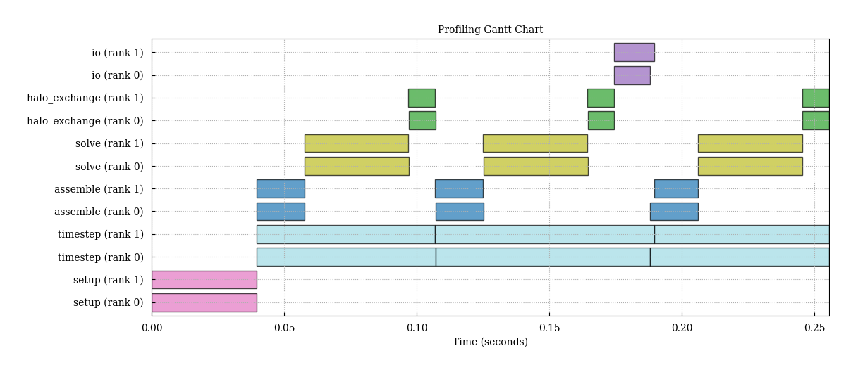
Both ranks appear by default, one lane per rank. Calls of the same
region share a color, and nested regions such as assemble and solve
get their own lanes rather than being drawn inside timestep — the
flame graph below is the view that shows the nesting.
Flame chart#
flame_plot.png answers when the calls happened instead. The call
stack is reconstructed from timestamp containment — a region whose
interval lies inside another’s is drawn one level above it:
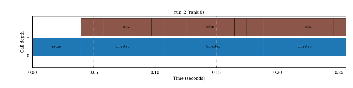
Like the Gantt chart, the flame chart is drawn per rank and defaults to
rank 0 only; pass --ranks to render more (one panel each). Both flame
views use the warm inferno colormap by default; override it with
--cmap when needed.
Flame graph#
flame_graph_plot.png aggregates repeated call paths. Its horizontal
axis is accumulated duration rather than wall-clock position, so it
shows where the recorded time went rather than when calls happened:
scope-profiler plot flame_graph profiling_data.h5 -o figures
Duration bar charts#
One bar chart is written per duration statistic. By default only total
time is shown; request other statistics with --metrics:
scope-profiler plot durations run_2.h5 -o figures
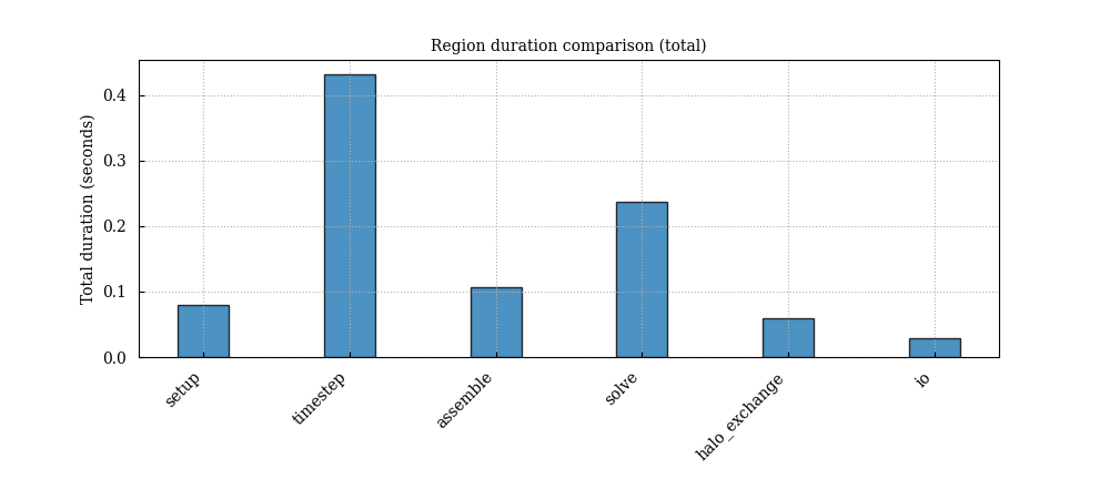
For example, --metrics avg total also writes an average-per-call
chart. With several input files, bars are grouped per region so runs can
be compared side by side.
Duration over time#
duration_timeseries_plot.png plots each region’s per-call duration
against wall-clock time, with a band spanning the minimum and maximum
across the selected ranks. Rank imbalance shows up as a widening band,
and slow drift (cache growth, memory pressure, throttling) as a trend:
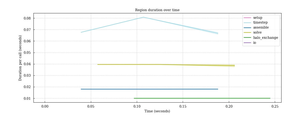
Here the middle timestep stands out, because that is the step that
also writes io. Regions called only once — setup and io in this
run — are a single point and stay invisible between the lines.
Comparing several runs#
Passing several files compares them. Each chart then either stacks one panel per file (Gantt, flame chart, flame graph) or groups the files together (durations), and a speedup plot is added:
scope-profiler plot default run_1.h5 run_2.h5 run_4.h5 -o figures_scaling
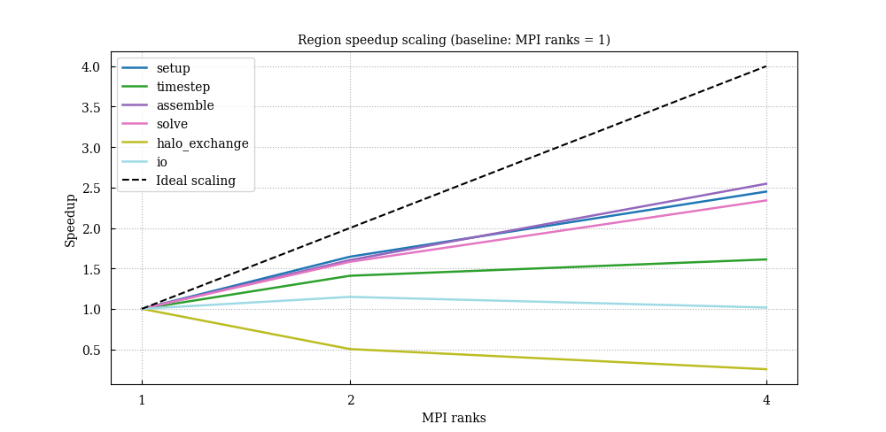
Each line is one region’s speedup relative to the smallest run, derived
from average per-call durations, against the dashed ideal-scaling line.
The mock solver behaves as designed: solve and assemble scale well,
io is serial and flat, and halo_exchange gets slower with more
ranks, dragging timestep below the ideal line.
The x-axis is the MPI rank count by default. --x switches it to
num_nodes, omp_num_threads or total_cores (all read from the run
metadata), or to any other metadata field — in which case the files stay
in the order given on the command line and no ideal-scaling line is
drawn:
scope-profiler plot speedup omp_*.h5 -o figures_scaling --x omp_num_threads
Files can also be selected with wildcards. Quote the pattern to let scope-profiler expand it rather than the shell:
scope-profiler plot default "runs/run_*.h5" -o figures_scaling
Naming the runs#
Each run is named after its label — set with
ProfileManager.setup(label=...), see Configuration — or, for
runs that set none, after its file’s stem. That name is what appears in
chart legends and panel titles, region_statistics.json and the
exported .prof / speedscope filenames.
--label overrides it for one invocation, once per file, in the order
the files are given:
scope-profiler plot default run_1.h5 run_2.h5 run_4.h5 -o figures_scaling \
    --label "1 rank" --label "2 ranks" --label "4 ranks"
The files themselves are not modified. Labels are free text; where one is used in a filename, spaces and other awkward characters become underscores.
Selecting which plots to generate#
Use a named plot kind for a single chart, or a preset for a common group:
# only the total-time bar chart and the speedup comparison
scope-profiler plot quick run_1.h5 run_2.h5 run_4.h5 -o figures

# just the Gantt chart, written to a specific file
scope-profiler plot gantt run_2.h5 -o gantt.png
Run scope-profiler plot list to see the available names. The built-in
presets are default (gantt and total durations), quick
(durations and speedup), and all (every plot except LIKWID unless
--metric is given).
Filtering regions and ranks#
--include and --exclude take regular expressions matched against
region names, and --ranks selects ranks — as individual values, dash
ranges, or a mix (0,2,4-7 expands to 0, 2, 4, 5, 6, 7):
scope-profiler plot gantt run_2.h5 -o figures_filtered \
    --include solve assemble \
    --ranks 0
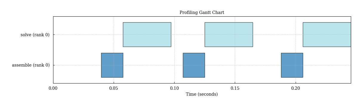
Filtering applies to every output of the run, including
region_statistics.json. On a large run it is also the quickest way to
make the charts readable again.
Region statistics JSON#
Whenever -o/--output is given, region_statistics.json is written
alongside the figures. It holds the numbers behind the charts: per-file,
per-region aggregates, the same statistics per rank, and the region
names common to all input files.
Each file’s label — the name it is given in chart legends here too —
is the one the run set with ProfileManager.setup(label=...), falling
back to the file’s stem for runs that set none.
{
  "units": { "durations": "seconds" },
  "filters": { "include": null, "exclude": null, "ranks": null },
  "common_regions": ["setup", "timestep", "assemble", "solve", "halo_exchange", "io"],
  "files": [
    {
      "label": "run_2",
      "file_path": "/scratch/run/run_2.h5",
      "num_ranks": 2,
      "region_statistics": {
        "setup": {
          "count": 2,
          "average_duration_seconds": 0.039551083,
          "min_duration_seconds": 0.0395205,
          "max_duration_seconds": 0.039581666,
          "std_duration_seconds": 3.0583e-05,
          "total_duration_seconds": 0.079102166,
          "per_rank": {
            "0": { "count": 1, "average_duration_seconds": 0.0395205, "...": "..." },
            "1": { "count": 1, "average_duration_seconds": 0.039581666, "...": "..." }
          }
        }
      }
    }
  ]
}
Interactive HTML charts#
--backend plotly renders the same charts as self-contained interactive
.html files instead of PNGs, with zooming and hover labels — useful
for long runs where a static Gantt chart becomes a smear. With --show,
the pages open in a browser:
scope-profiler plot default run_2.h5 -o figures_html --backend plotly
Hovering any bar, point, cell or flame frame shows the summary of the
region it belongs to — the same statistics Region.get_summary()
reports (calls, total, self, average, min, max, first, last, std, and
the GPU totals when there are any), plus what identifies the thing under
the cursor: the hovered call’s own start and duration on the Gantt
chart, the bin on the histogram, the run behind a scaling point. A bar
showing one rank’s data is described by that rank’s region; a bar pooled
over ranks by the pooled one. A --combine-regions bar has no single
region behind it, so it lists its members and their pooled statistics
instead.
The matplotlib backend (the default) writes .png and needs no extra
dependency; the Plotly backend writes .html and likewise needs nothing
beyond Plotly itself.
Build a chart in your own site#
@scope-profiler/plotly turns the JSON written by export plot-data
into a plain Plotly { data, layout } figure. It does not bundle
Plotly, so a site can choose its own Plotly build and renderer. This
live example is rendered by the published npm package in the
documentation page itself:
npm install @scope-profiler/plotly plotly.js-dist-min
The same pattern works with real output:
import Plotly from "plotly.js-dist-min";
import { buildGanttFigure, renderFigure } from "@scope-profiler/plotly";

const payload = await fetch("/figures/gantt_data.json").then((response) => response.json());
await renderFigure(Plotly, document.querySelector("#gantt"), buildGanttFigure(payload));
See Plotly figures for the web for Gantt, durations, flame, and speedup examples.
For terminal-friendly simple plots, use Plotext 6:
scope-profiler plot durations run_2.h5 --backend plotext -o durations.txt
Plotext writes plain text and is intentionally limited to simple duration, scaling, histogram, and imbalance plots; use Matplotlib or Plotly for Gantt, flame, heatmap, and hardware-counter visualizations.
PyVis renders the interactive callgraph only; it cannot render
timeline or flame charts. For example, use
scope-profiler plot callgraph run.h5 --backend pyvis, or choose
Matplotlib/Plotly for flame_chart or flame_graph.
Exporting the data behind the charts#
scope-profiler export plot-data writes the exact series each chart was
drawn from, so the figures can be reproduced — or re-styled elsewhere —
without the HDF5 files:
scope-profiler export plot-data run_2.h5 -o data
gantt_data.csv                    file, rank, region, start_seconds, end_seconds
flame_data.csv                    file, rank, call_id, parent_call_id, region, call_path,
                                  source_file, source_lineno, depth, start_seconds, end_seconds,
                                  inclusive_duration_seconds, exclusive_duration_seconds
durations_data.csv                file, region, metric, value_seconds
duration_timeseries_data.csv      file, region, call_index, time_seconds,
                                  mean/min/max_duration_seconds, num_ranks
speedup_data.csv                  only when several files are passed
file,rank,region,start_seconds,end_seconds
run_2,0,setup,0.000202333,0.039720250
run_2,1,setup,0.0,0.038490875
run_2,0,timestep,0.039737417,0.106206750
--format json writes JSON instead, including a colors map matching
the colors used in the plots, so a re-rendered chart keeps the same
region colors. Gantt, flame and roofline data also carry file_ranks,
each run’s rank count: plots name a rank - solve (rank 0) - only for a
run with more than one, and the @scope-profiler/plotly builders follow
the same rule. Gantt JSON intervals also carry depth, the call’s
nesting level (0 for a top-level call), when the rank’s calls nest; the
builders’ maxDepth and topN options use it to hide nested calls and
keep the most expensive regions.
scope-profiler export plot-data run_2.h5 -o data --format json
Exporting to external profile viewers#
scope-profiler export also writes the run in formats other tools
understand:
# cProfile/pstats format, one file per exported rank
scope-profiler export prof run_2.h5 -o figures
snakeviz figures/profile_rank0.prof

# speedscope, one file holding one profile per exported rank
scope-profiler export speedscope run_2.h5 -o figures
npx speedscope figures/profile.speedscope.json
Both reconstruct the call graph from region nesting the same way the
flame graph does, and both export only the ranks selected with --ranks
(rank 0 by default). CLI reference documents what that reconstruction
implies for partially overlapping regions and recursion.
The .prof export preserves reconstructed call paths for SnakeViz: a
solve region reached through assembly and one reached through
postprocess appear as assembly > solve and postprocess > solve
respectively. This makes the tree larger, but prevents different call
sites from being conflated.
Files without timing data#
A run that entered no region records nothing to plot. Rather than
failing inside the plotting code, plot reports what is there and
stops:
No timing data found — these files recorded no calls.

empty_run.h5:
Reproducing the figures on this page#
python examples/generate_cli_docs_figures.py
The script runs the mock solver at 1, 2 and 4 ranks (via mpirun, if
available), invokes the plot commands shown above, and copies the
resulting PNGs into figures/cli/, which the docs build picks up as
_static/figures/cli/. Pass --keep DIR to also keep the HDF5 files
and the raw CLI output around.