Profiling overhead#

Install for this page: pip install "scope-profiler[pproc]"; the benchmark uses maxplotlib to save its result as a figure.

scope-profiler is designed for production HPC workloads where instrumentation must not distort the measurements. This page documents the per-call overhead of each profiling mode.

Benchmark#

The benchmark script (examples/benchmark_overhead.py) times a small workload function through each profiling mode and subtracts the bare function-call baseline to isolate the overhead.

python examples/benchmark_overhead.py          # save figure
python examples/benchmark_overhead.py --show   # display interactively

Profiling overhead by regiontype

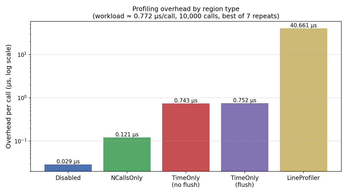
Results summary#

Region type	Overhead / call
Disabled	~0.1 µs
TimeOnly	~0.33 µs
LineProfiler	~50 µs

(Numbers measured on an Apple M-series CPU; absolute values will vary, but the relative ordering is stable.)

What this means for HPC#

The TimeOnly mode — the default and most commonly used — adds roughly 0.33 µs per instrumented call. In practice:

A 64×64 matrix multiply takes ~36 µs, so the overhead is < 2 %.
A 256×256 matrix multiply takes ~780 µs, giving < 0.1 % overhead.
Typical simulation time steps run for milliseconds or longer, making the overhead unmeasurable.

The profiler can also be fully deactivated at startup (deactivate_profiling=True) without removing any instrumentation from the source code. In this mode the overhead drops to ~0.1 µs — barely above the cost of a bare function call.

LineProfiler#

The line_profiler mode is intentionally heavier (~50 µs per call) because it instruments every source line in the profiled function. It is meant for targeted debugging of individual functions, not for always-on use in hot loops.

Regression guards#

The numbers above are benchmarks. What keeps them from drifting is a separate set of budgets in the test suite, run with the overhead marker:

pytest -m overhead                 # per-call, write, and read budgets
pytest -s -m overhead              # ...printing every measurement
pytest src/scope_profiler/tests/test_storage_size.py -s   # file size

module	covers
`test_overhead.py`	per-call cost of each region type, region lookup, source capture, buffer growth, nesting depth
`test_overhead_io.py`	`finalize()` write cost, publication packing, read cost, summary-only reads, the timestamp codec
`test_storage_size.py`	bytes per event, the fixed floor, scaling in events/ranks/regions, compression ratios

The budgets sit roughly an order of magnitude above what an idle laptop measures, so a loaded CI machine still passes while a structural regression — an allocation or a lock on the hot path, a per-event Python loop in the writer, a quadratic index rebuild — does not. Each measurement takes the minimum over several repeats, which is the robust estimator for a cost: noise can only ever add time.

The scaling assertions matter more than the absolute ones, and are the reason the suite catches things a benchmark would not. An absolute budget can only catch a change large enough to blow it; a ratio between the same measurement at two sizes catches a change in the shape of the cost. For example, a summary-only read of a ten-times-larger profile must cost about the same (measured: 1.0x), which is what proves it never touches the event columns.

Writing and reading a profile#

The per-call numbers above are what instrumentation adds to the program. What finalize() then spends turning the recorded buffers into a file is separate, and matters for its own reasons: it happens at the end of a run that may have been queued for hours, and under MPI it is collective, so a write that scales badly stalls every rank.

Measured on an idle laptop, jittered synthetic data:

	cost
write, 100,000 events	~93 ns/event
write, 10,000 events	~510 ns/event
write with `hdf5_compression="auto"`	~2x the plain write
publication packing, small profile	~2.5 ms (fixed)
read, uncompressed	~18 ns/event
read, gzip-compressed	~66 ns/event
summary-only read	independent of event count
timestamp encode / decode	~0.4 / ~2.1 ns/event

examples/benchmark_io.py measures all of these, and --scaling sweeps the rank count so the per-rank cost can be checked for flatness:

python examples/benchmark_io.py --scaling 8,32,128
python examples/benchmark_io.py --json          # to diff between revisions

A small profile is dominated by the fixed ~2.5 ms publication pass, which is why the per-event figure is so much higher at 10,000 events than at 100,000. That pass is what removes the per-dataset chunk overhead; see Output file size.

Reading through gzip costs about 3.5x an uncompressed read. That is the other side of the ~5x space saving, and it is why compression is opt-in rather than the default.

Where the time goes#

A recorded call is two perf_counter_ns() reads (~33 ns each from Python) plus a slot reservation; the rest is the cost of the with statement or the decorator wrapper itself. Those two together are about half the total and are out of the library’s hands: an empty with on a Python object already costs ~109 ns, and on a C-implemented one ~76 ns. Nothing touches the filesystem: the timestamps accumulate in a numpy buffer that doubles when it fills, and the whole buffer is written once, at finalize(). Writing is therefore not part of the per-call cost at all — deactivate_file_output changes what happens at the end of the run, not what happens in the loop.

Profiling overhead

Contents