Configuration#
Install for this page:
pip install scope-profiler. The compression section additionally needspip install "scope-profiler[compression]".
All profiling behaviour is controlled through ProfileManager.setup().
Decorators and disabled regions may be declared before setup; they
become active when setup installs the run configuration. Calls made on
the ProfileManager class use its process-wide default configuration.
Independent ProfileManager() instances each have their own
configuration and regions; see Multiple sessions.
For a script that should finalize automatically on normal interpreter exit, opt in explicitly:
import scope_profiler as sp

sp.setup(file_path="run.h5", auto_finalize=True)
An explicit finalize() cancels the pending exit hook. Avoid automatic
finalization for MPI programs whose ranks may not exit together; use
session() or coordinated explicit finalization there.
Multiple sessions#
Instantiate a manager when two profiling sessions need to coexist. Calls must be made through the manager that should receive the event:
from scope_profiler import ProfileManager

compute_profiler = ProfileManager()
io_profiler = ProfileManager()

with compute_profiler.session(file_path="compute.h5", verbose=False):
    with io_profiler.session(file_path="io.h5", verbose=False):
        with compute_profiler.region("solve"):
            solve()
        with io_profiler.region("checkpoint"):
            write_checkpoint()
The class-level API remains available as the default manager and is
isolated from instantiated managers. Decorators are isolated in the same
way: use @compute_profiler.profile(...) to attach a function to that
session.
The sessions above coexist by nesting distinct managers in one execution
thread. Setting up and finalizing a session is still a single-threaded
operation: do not enter or finalize profiling sessions concurrently from
Python threads. Profiling regions from several threads is supported —
see Threads, tasks and coroutines — but that is a property of track_threads, not
of multiple managers.
Multiple sessions also do not isolate process-global instrumentation
backends. In particular, LIKWID owns one marker state per process, so
only one overlapping manager may use use_likwid=True. Timing-only,
aggregation, line-profiling, GPU-timing, and NVTX configurations retain
their existing behavior.
ProfileManager.setup() parameters#
Parameter |
Type |
Default |
Description |
|---|---|---|---|
|
|
|
Master switch. When |
|
|
|
Finalize once at normal interpreter exit unless finalized explicitly first. |
|
path or |
unset |
Direct output destination; format follows the extension, while |
|
|
|
Explicitly replace a configuration that is still active. |
|
|
|
Wrap regions with LIKWID marker API calls for hardware counter collection. Requires |
|
|
|
Collect selected Linux |
For the richer counter backend, install scope-profiler[perf-events].
It uses py-perf-event when every selected event is supported by that
package and falls back to the built-in Linux syscall backend otherwise.
Both routes remain subject to the host’s perf_event_paranoid policy.
If a host reports permission denied, an administrator can grant normal
users access for the current boot with
sudo sysctl -w kernel.perf_event_paranoid=1. Run the profiled program
as its ordinary user afterwards; sudo python uses a separate Python
environment and commonly cannot import the project or its optional
dependencies. | use_line_profiler | bool | False | Enable
line-by-line profiling via line_profiler. See Line-by-line profiling. |
| use_memray | bool | False | Record process-wide allocations
in a native Memray capture. Requires scope-profiler[extras]. | |
memory_profile_path | str or None | None | Memray capture
path; defaults to <file-stem>.memray.bin. | | use_nvtx | bool
| False | Add NVTX ranges for NVIDIA Nsight tools; requires
scope-profiler[nvtx]. | | recursive_profile | bool | False
| Enable recursive nested-call profiling for all decorated functions by
default. | | deactivate_file_output| bool | False | When
True, write no HDF5 file at all; the run stays in memory. See below.
| | buffer_limit | int | 1024 | Initial per-region buffer
capacity. Buffers grow on demand, so this is a starting size, not a cap.
| | file_path | str | "profiling_data.h5" | Output path for
the merged HDF5 file written by finalize(). | | output_mode |
str | "auto" | MPI writer: parallel HDF5 when available, otherwise
direct token-ordered writes. Accepts auto, direct, or parallel. |
| hdf5_compression | str or None | None | Compress
timestamp, GPU-duration, and line-profile arrays with gzip, lzf,
optional zstd, or auto to compress only runs large enough to repay
the write CPU. | | hdf5_compression_level | int or None |
None | GZIP level 0–9 or Zstandard level 1–22. LZF has no level. |
| hdf5_chunk_size | int or None | None | Maximum events per
HDF5 chunk; enables chunked partial reads even without compression. |
| label | str | None | Short name for the run, used by
post-processing wherever a run has to be named. See below. | |
capture_region_source| bool | False | Record where each region
is defined (see HDF5 output & post-processing from Python). Off by default; see below
for its cost and how to turn it on. | | metadata_detail | str |
"minimal" | How much of the environment is recorded: "minimal"
(versions, platform, CPU, rank/thread counts), or "full" to add user,
host, directories, environment variables and SLURM_*. See
HDF5 output & post-processing from Python. | | aggregation_mode | bool |
False | Keep only count, total, minimum, maximum, and exclusive total
per region; individual timeline events are unavailable. | |
track_threads | bool | False | Give every thread its own
buffers and lane, and describe every thread the run touched. See
Threads, tasks and coroutines. | | track_async | bool | False | Also
follow asyncio tasks and greenlets, and record the await time of every
call. Implies track_threads. |
Grouping settings, and reusing them#
The settings in the table above are also the fields of
ProfilingOptions, which holds a set of them so they can be built away
from the call site and reused across runs:
from scope_profiler import ProfileManager, ProfilingOptions

options = ProfilingOptions(use_likwid=True, buffer_limit=8192)

ProfileManager.setup(options=options, file_path="run_a.h5")
ProfileManager.setup(options=options, file_path="run_b.h5")
A keyword argument passed alongside options wins over the same field
on it, which in turn wins over a config_path TOML file.
The settings that share a prefix - the Memray, GPU and HDF5 ones - can also be given as groups, which spell them without the prefix:
from scope_profiler import GPUOptions, HDF5Options, MemrayOptions, ProfilingOptions

options = ProfilingOptions(
    file_path="run.h5",
    hdf5=HDF5Options(compression="gzip", compression_level=4, chunk_size=65_536),
    memray=MemrayOptions(enabled=True, native_traces=True),
    gpu=GPUOptions(timing=True, backend="torch"),
)
The two spellings configure identical runs; setting one thing both ways
raises ValueError rather than picking a winner.
Settings in a TOML file#
setup(config_path=...) reads the same settings from a [profiling]
table, flat or grouped into the matching sub-tables:
[profiling]
file_path = "run.h5"
buffer_limit = 8192

[profiling.hdf5]
compression = "gzip"
compression_level = 4
An unrecognised setting is an error naming the closest real one, in the
file and at the setup() call alike.
Output file size#
Three things decide how large a profile is, and the defaults are chosen to keep the write cheap rather than the file small.
Small profiles are packed on publication. HDF5 gives every growable dataset chunked storage, and a full chunk plus its index is allocated as soon as the first element is written — which for a profile with a handful of events is the file. The finished file is rewritten with those datasets stored contiguously, which takes a one-region run from 193 KiB to 17 KiB. Nothing to configure; files too large for it to matter are left alone.
Timestamps are stored as gaps and durations. A region’s calls are recorded as the gap since its previous call and the duration of each call, rather than two absolute nanosecond timestamps. The information is identical — the first value of each run is absolute — but the numbers are ~15 bits instead of ~60, which is most of what makes compression effective here.
Compression is opt-in. hdf5_compression="auto" compresses a run
once it is large enough for the saving to repay the write CPU, and
leaves small ones alone:
ProfileManager.setup(hdf5_compression="auto")
What a profile actually costs#
Two numbers describe any profile: a fixed cost that does not depend on the run, and a marginal cost per recorded call.
size |
|
|---|---|
fixed floor (one region, one call) |
~15.7 KiB |
per event, uncompressed |
~16.3 bytes |
per event, |
~3.1 bytes |
The floor is HDF5’s own bookkeeping for the ~15 objects the schema uses — object headers, group tables, the region dictionary. It does not grow with the region count (10 regions cost the same as 1), and it is what dominates a profile of a few hundred calls.
The marginal cost is two int64 per call and essentially nothing else:
16.3 measured against 16 bytes of information stored. That holds as the
run grows in events, in ranks, and in regions — a profile with 200
regions costs about 1.3x one with 2 regions holding the same number of
events, because a region costs one index row rather than anything per
call.
Measured end to end on a 100,000-event profile, against 3313 KiB for the same run before any of this:
size |
||
|---|---|---|
default |
3180 KiB |
1.0x |
|
142 KiB |
23x |
Compression ratios depend on the data. That 23x is a real profile, whose gaps between calls are small and regular. On deliberately jittered synthetic data — the pessimistic case — the same setting gives ~5x, and the delta encoding on its own accounts for ~1.4x of it against absolute timestamps at the same filter. A real profile is closer to the former.
aggregation_mode=True is smaller still, and is the only option whose
size does not grow with the call count at all: it records no timeline,
so 10,000 calls cost exactly what 10 do.
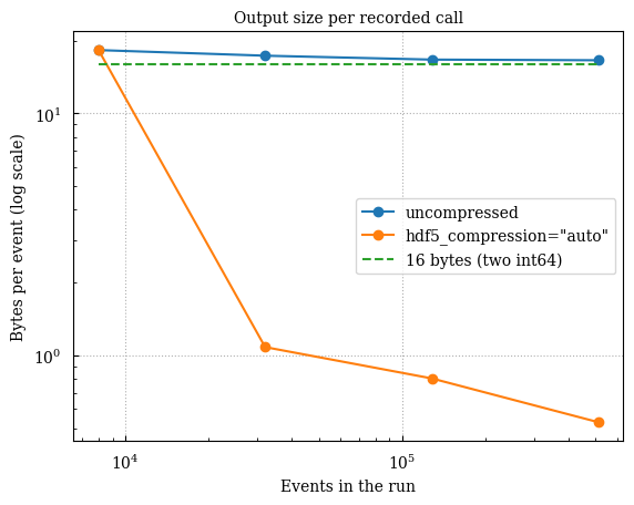
The shape is what the table cannot show. Uncompressed, the curve falls
from the fixed cost of an almost-empty file onto the flat 16 bytes a
call actually stores. Compressed, it steps down sharply once the run
crosses the threshold at which "auto" starts applying a filter — below
it the two curves are the same file. Regenerate it with:
python examples/benchmark_io.py --scaling 2,8,32,128 --figure figures
That script also reports the write and read cost of compression alongside the space it saves, since the space is only worth it against those.
These figures are asserted, not just documented. test_storage_size.py
builds profiles from fixed synthetic arrays — file size is
deterministic, unlike a timing — so its budgets are tight enough to
catch a lost encoding or a third column per call immediately. See
Profiling overhead for how that fits
with the timing budgets.
HDF5 compression and chunking#
The default remains contiguous and uncompressed, which minimizes write CPU cost for small profiles. Large traces can trade some CPU time for smaller files and chunk-addressable reads:
ProfileManager.setup(
    hdf5_compression="gzip",
    hdf5_compression_level=4,
    hdf5_chunk_size=65_536,
)
gzip is portable across HDF5 installations and usually gives the
smallest files of the built-in filters. lzf is faster but generally
compresses less. Both use HDF5’s byte-shuffle filter, which is
particularly effective for nearby int64 timestamps. Zstandard is
available through the optional filter plugin:
pip install "scope-profiler[compression]"
ProfileManager.setup(
    hdf5_compression="zstd",
    hdf5_compression_level=3,
    hdf5_chunk_size=65_536,
)
Readers of a Zstandard-compressed file must also have hdf5plugin
installed so HDF5 can load the filter. Compression automatically makes
datasets chunked; set only hdf5_chunk_size when partial reads are
desired without compression. In MPI auto mode, scope-profiler uses the
direct single-file writer if the parallel HDF5 library lacks the
requested filter. Explicit output_mode="parallel" instead fails early
with a diagnostic, so a parallel-HDF5 test cannot silently exercise the
direct backend.
Enabling capture_region_source#
Every Python region records just its defining filename and line number for decorators and direct context-manager regions, using a one-time frame/code-object lookup. It neither reads nor parses source files and adds no per-call work.
Off by default, because its cost - while cheap for a typical file - is not always. Capturing a region’s source parses its defining file’s AST and walks it once per distinct file, the first time any of its regions is created – not once per region, and not on any later call. Measured cost tracks that file’s total size, not the size or number of the regions it defines:
File |
Cost, 1 rank |
Cost per rank, 64 ranks (shared, oversubscribed node) |
|---|---|---|
Typical, a few hundred lines |
< 1 ms |
a few ms |
~10,000 lines, ~1,000 regions (one spanning 3,000 lines) |
~0.3 s |
~2.9 s |
The per-region text itself is cheap to extract even when huge (~0.1 ms for a 3,000-line block) - the file-wide parse dominates. Every rank pays this independently and concurrently, so on a job with more ranks than idle cores it compounds under contention; at rank counts within the idle core count (1–8 ranks, above), it stays flat. For a typical, modestly sized codebase this is negligible either way - turn it on with:
ProfileManager.setup(capture_region_source=True)
Naming a run with label#
Post-processing names a run after its output file: run_a.h5 becomes
run_a in chart legends, summary headings and the JSON statistics.
label overrides that with something you choose:
ProfileManager.setup(file_path="run_a.h5", label="128 ranks")
The label is stored as metadata in the output file, so it survives into
every later step — scope-profiler plot, scope-profiler inspect, the
plotting functions and the exporters all pick it up with no extra flags.
It is especially worth setting for scaling studies, where a legend
reading 128 ranks beats one reading run_a.
Reading it back, results.label is the label or None, while
results.display_label is the label or the file stem — what
post-processing actually prints.
Profiling modes#
Every active region records nanosecond timestamps; the remaining flags
decide what it records on top of them. This strategy dispatch
picks the region class once, at setup(), so there are no runtime
conditionals in the hot path:
Flags |
Region class |
What it records |
|---|---|---|
|
|
Nothing (profiling off) |
(defaults) |
|
Timestamps |
|
|
Timestamps + LIKWID |
|
|
Timestamps + line-by-line |
|
|
Timestamps + NVTX ranges |
use_line_profiler=True takes precedence over use_likwid=True.
use_nvtx=True adds NVTX annotations while retaining the normal CPU
timing records. NVTX does not measure GPU kernel duration itself; use
NVIDIA Nsight Systems/Compute or CUDA events for device-side timings.
use_likwid=True and use_nvtx=True are currently separate modes, with
LIKWID taking precedence.
deactivate_file_output is not part of this dispatch: recording is
identical either way, and the flag only decides whether finalize()
writes the buffers out. With deactivate_file_output=True, use
finalize(return_results=True) to get the recorded data back — see the
Python API
guide.
What is no longer configurable#
Two things used to be options and are now decided for you, because there was only ever one sensible answer:
The run’s start time is the moment
setup()is called. It is stored as thestart_time_nsmetadata field and is the origin of the relative timeline in post-processing.MPI is used exactly when the process was started by an MPI launcher (
mpirun,mpiexec,srun, …), so a plainpython script.pynever importsmpi4py. SetSCOPE_PROFILER_MPI=0or=1in the environment to overrule the detection.
Toggling profiling at runtime#
With the default class-level manager, you can leave all instrumentation in place and simply flip the master switch:
import os
from scope_profiler import ProfileManager

ProfileManager.setup(
    deactivate_profiling=os.environ.get("DISABLE_PROFILING", "0") == "1",
)
Recursive profiling of decorated entrypoints#
Set recursive_profile=True to record Python function calls made inside
decorated functions:
ProfileManager.setup(recursive_profile=True)

@ProfileManager.profile("entry")
def entry():
    compute_step()
You can override this per function with
@ProfileManager.profile(..., recursive=False) or
@ProfileManager.profile(..., recursive=True).
When deactivate_profiling=True, every region is a
DisabledProfileRegion whose __enter__ / __exit__ / wrap are
trivial no-ops, adding only the cost of a Python function call (~0.1
µs).
Re-configuring#
After a run has been finalized, calling setup() starts a fresh session
with new configuration. Calling it while a run is still active raises an
error; pass replace=True when intentionally replacing that active run:
ProfileManager.setup(file_path="run_a.h5")
# ... profile some code ...
ProfileManager.finalize()

# Start a fresh session with different settings
ProfileManager.setup(file_path="run_b.h5", use_line_profiler=True)
# ...
ProfileManager.finalize()
GPU timing and synchronization#
Enable CUDA-event timing to measure asynchronous device work:
ProfileManager.setup(
    use_gpu_timing=True,
    gpu_timing_backend="cupy",  # or "torch"
    gpu_sync_on_exit=True,     # optional; defaults to False
)
gpu_sync_on_exit=True waits for the current device after recording
each region’s GPU end event and before recording its CPU end time. It
applies to context managers and decorators, including exceptional exits.
This includes the wait in CPU durations and removes CPU/GPU overlap,
changing the workload being measured. The wait can also include work
queued before the region or on other streams; it is not an isolated
kernel timing. GPU events continue to measure the backend’s current
stream. Synchronization requires use_gpu_timing=True; custom backends
must implement synchronize().
The grouped equivalent is
GPUOptions(timing=True, backend="cupy", sync_on_exit=True), or in
TOML:
[profiling.gpu]
timing = true
backend = "cupy"
sync_on_exit = true
inspect, HTML report, and the end-of-run summary automatically add
gpu total [s] and gpu avg [s] when selected regions have GPU
timings. Explicit column selections can include gpu_total and
gpu_avg. GPU averages use only calls with GPU measurements. CPU-only
regions show a dash. A warning flags GPU totals over twice the CPU total
as possible asynchronous enqueue timing. Nested totals are inclusive.
Compare device timings with:
scope-profiler diff baseline.h5 candidate.h5 --metric gpu_total
scope-profiler diff baseline.h5 candidate.h5 --metric gpu_avg