Quickstart#
Install for this page:
pip install "scope-profiler[pproc]". The base install is sufficient through the text summary;pprocadds the plotted example in step 4.
This page walks through the lowest-touch workflow first: mark regions, run, and inspect. It then shows the equivalent Python lifecycle API.
1. Run an instrumented script#
Add regions where the application has meaningful phases; no in-source session or setup call is required:
import scope_profiler as sp

def main():
    with sp.region("iteration", tags=["solver"]):
        evolve()

main()
Run the script through the CLI:
scope-profiler run example.py -o profile.h5
The same script run with python example.py leaves the regions disabled
and writes no profile. To trace functions that were not explicitly
marked, opt in to recursive tracing:
scope-profiler run --recursive example.py
You can select tagged regions and filter recursive function names without editing the script again:
scope-profiler run --tag solver --include 'my_app.*' example.py
For a named application entrypoint, use --entrypoint main.
2. Start a session#
Use ProfileManager.session() as the default entry point. Configuration
arguments are passed directly to the session:
from scope_profiler import ProfileManager

with ProfileManager.session():
    # Profile regions inside this block.
    run_application()
All regions created inside the session — even in other modules — share its configuration.
For a callable entrypoint, sp.run() provides the same setup/finalize
safety without a context-manager block:
import scope_profiler as sp

sp.run(run_application, output="profile.h5")
Use sp.setup(auto_finalize=True) when a long-running script needs one
startup call and cannot wrap its whole application in a with block.
3. Instrument your code#
Decorator#
Use @ProfileManager.profile to wrap an entire function:
@ProfileManager.profile("matrix_multiply")
def matrix_multiply(a, b):
    return a @ b
The decorator also works without an explicit name — it uses the function name by default:
@ProfileManager.profile
def matrix_multiply(a, b):
    return a @ b
To include nested Python calls made by a decorated function:
with ProfileManager.session(recursive_profile=True):
    @ProfileManager.profile("solver_step")
    def solver_step():
        return advance_state()  # nested calls are recorded automatically
Context manager#
Use ProfileManager.region() for finer-grained control:
for step in range(num_steps):
    with ProfileManager.region("time_step"):
        evolve(state, dt)

    with ProfileManager.region("io"):
        write_checkpoint(state)
The two styles can be mixed freely.
4. Finish the session#
When the with block exits, the session writes all buffered data,
merges per-rank HDF5 files, and prints a summary. Use
return_results=True to keep the finalized results in memory:
with ProfileManager.session(return_results=True) as run:
    run_application()

results = run.results
Output:
  ╭─────────────────────────────────────────────────────────╮
  │ region                       % session      total [s]   │
  ├─────────────────────────────────────────────────────────┤
  │ scope_profiler.session       100.00%        0.002876    │
  │ └─ (own)                        45.51%         0.001309 │
  │ └─ matrix_multiply (100x)       5.03%          0.000145 │
  │ └─ time_step (1kx)              49.46%         0.001422 │
  ╰─────────────────────────────────────────────────────────╯

  ╭─ Info ─────────────────────────────────────────────────────────────────────────────────────────────────────────────────────────────╮
  │ Summary: profiling_data.h5  (1 rank(s))                                                                                            │
  │                                                                                                                                    │
  │ Explore:                                                                                                                           │
  │   Inspect: scope-profiler inspect ../../../../../../tmp/scope-profiler-docs-output-bymi532c/profiling_data.h5                      │
  │   TUI:     scope-profiler tui ../../../../../../tmp/scope-profiler-docs-output-bymi532c/profiling_data.h5                          │
  │                                                                                                                                    │
  │ Visualize and export:                                                                                                              │
  │   Plot:    scope-profiler plot default ../../../../../../tmp/scope-profiler-docs-output-bymi532c/profiling_data.h5 -o plots --show │
  │   Report:  scope-profiler report ../../../../../../tmp/scope-profiler-docs-output-bymi532c/profiling_data.h5 -o report.html        │
  │   Export:  scope-profiler export plot-data ../../../../../../tmp/scope-profiler-docs-output-bymi532c/profiling_data.h5 -o data     │
  │   Lines:   scope-profiler line-profile ../../../../../../tmp/scope-profiler-docs-output-bymi532c/profiling_data.h5                 │
  │                                                                                                                                    │
  │ Compare runs:                                                                                                                      │
  │   Diff:    scope-profiler diff BASE.h5 CANDIDATE.h5                                                                                │
  │   Check:   scope-profiler check BASE.h5 CANDIDATE.h5                                                                               │
  │                                                                                                                                    │
  │ Durations are in seconds.                                                                                                          │
  │ Regions may nest, so the summed total can exceed the wall-clock time.                                                              │
  │ % session uses wall-clock coverage; overlapping recursive calls count once.                                                        │
  ╰────────────────────────────────────────────────────────────────────────────────────────────────────────────────────────────────────╯
The same table is available from ProfilingResults.print_summary() and
from scope-profiler inspect; pass verbose=False to finalize() to
suppress it.
5. Inspect the data#
After finalization the timing data is saved to profiling_data.h5
(default). Use the built-in CLI to generate a Gantt chart:
scope-profiler plot default profiling_data.h5 --show
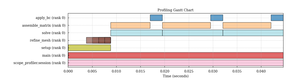
See Plotting with the CLI for the other charts and exports it can produce. Or load the data programmatically:
from scope_profiler import load

results = load("profiling_data.h5")

# The quickest look: a summary table of every region.
results.print_summary()

# Or region by region (durations are in seconds).
for region in results:
    print(f"{region.name}: {region.num_calls} calls, "
          f"avg {region.average_duration:.4f} s")
load() reads whichever format the file is in — HDF5 or JSON — so a
path is all you need. read_h5() and read_json() remain available
when the format is already known.
Complete example#
from scope_profiler import ProfileManager

with ProfileManager.session():
    @ProfileManager.profile("main")
    def main():
        x = 0
        for i in range(10):
            with ProfileManager.region("iteration"):
                x += 1

    main()
python example.py
  ╭────────────────────────────────────────────────────────╮
  │ region                    % session      total [s]     │
  ├────────────────────────────────────────────────────────┤
  │ scope_profiler.session    100.00%        0.000230      │
  │ └─ (own)                     39.01%         0.000090   │
  │ └─ main                      60.99%         0.000141   │
  │ │ └─ (own)                     53.66%         0.000124 │
  │ │ └─ iteration (10x)           7.33%          0.000017 │
  ╰────────────────────────────────────────────────────────╯

  ╭─ Info ─────────────────────────────────────────────────────────────────────────────────────────────────────────────────────────────╮
  │ Summary: profiling_data.h5  (1 rank(s))                                                                                            │
  │                                                                                                                                    │
  │ Explore:                                                                                                                           │
  │   Inspect: scope-profiler inspect ../../../../../../tmp/scope-profiler-docs-output-bymi532c/profiling_data.h5                      │
  │   TUI:     scope-profiler tui ../../../../../../tmp/scope-profiler-docs-output-bymi532c/profiling_data.h5                          │
  │                                                                                                                                    │
  │ Visualize and export:                                                                                                              │
  │   Plot:    scope-profiler plot default ../../../../../../tmp/scope-profiler-docs-output-bymi532c/profiling_data.h5 -o plots --show │
  │   Report:  scope-profiler report ../../../../../../tmp/scope-profiler-docs-output-bymi532c/profiling_data.h5 -o report.html        │
  │   Export:  scope-profiler export plot-data ../../../../../../tmp/scope-profiler-docs-output-bymi532c/profiling_data.h5 -o data     │
  │   Lines:   scope-profiler line-profile ../../../../../../tmp/scope-profiler-docs-output-bymi532c/profiling_data.h5                 │
  │                                                                                                                                    │
  │ Compare runs:                                                                                                                      │
  │   Diff:    scope-profiler diff BASE.h5 CANDIDATE.h5                                                                                │
  │   Check:   scope-profiler check BASE.h5 CANDIDATE.h5                                                                               │
  │                                                                                                                                    │
  │ Durations are in seconds.                                                                                                          │
  │ Regions may nest, so the summed total can exceed the wall-clock time.                                                              │
  │ % session uses wall-clock coverage; overlapping recursive calls count once.                                                        │
  ╰────────────────────────────────────────────────────────────────────────────────────────────────────────────────────────────────────╯