HDF5 output & post-processing from Python#
Install for this page:
pip install "scope-profiler[pproc]"enables all examples. Reading HDF5 and inspecting regions need only the base install; pandas DataFrames and plotting needpproc.
Unless deactivate_file_output=True, finalize() writes the run’s
timing data into a single HDF5 file. Under MPI, ranks write their own
event arrays directly through parallel HDF5 or token-ordered access.
This page covers the file layout and the Python API for reading and plotting it. The same charts are available from the command line without writing any code — see Plotting with the CLI.
HDF5 file structure#
The merged output file (default: profiling_data.h5) has the following
layout:
profiling_data.h5
├── metadata/                  (attributes describing the run)
├── region_table/
│   └── names                 (region ID → UTF-8 name)
├── rank_region_index/
│   ├── region_ids, ranks
│   ├── event_offsets, event_counts
│   ├── summary_statistics   (fixed-size per-rank/region statistics)
│   └── source_files, source_lines, source_texts, tags
├── events/
│   ├── start_times           (int64, nanoseconds)
│   ├── end_times             (int64, nanoseconds)
│   ├── gpu_durations         (optional int64, -1 means unavailable)
│   ├── thread_ids            (optional int64, -1 means unknown)
│   ├── task_ids              (optional int64, -1 means "outside any task")
│   └── await_ns              (optional int64, nanoseconds suspended)
├── thread_table/             (optional; one row per thread, per rank)
├── task_table/               (optional; one row per asyncio task or greenlet)
└── rank<N>/                  (only auxiliary line-profile/LIKWID records)
The root attribute scope_profiler_schema identifies the HDF5 layout
version. New files currently use schema version 3. Files created
before this attribute was introduced are treated as version 1 for
backward compatibility; files from a newer, unsupported schema are
rejected with an upgrade hint.
Region names are stored once. Each rank/region pair indexes a contiguous slice of the shared event columns, avoiding thousands of small HDF5 objects.
Timestamps are stored as int64 nanoseconds from
time.perf_counter_ns().Runs with
track_threads=Trueadd thethread_idsevent column and thethread_tablegroup;track_async=Trueaddstask_ids,await_nsandtask_table. The two tables describe what those per-call columns index into. A run without them writes none of the four, which is how a reader tells “single-threaded” from “threads not recorded”. See Threads, tasks and coroutines.Runs with
use_likwid=Trueadditionally get arank<N>/likwid/group holding the hardware counters and derived metrics of every marker region. See LIKWID hardware counters.
Run metadata#
Every file records the environment it was produced in, as attributes on
the metadata group. This is what lets you tell two otherwise identical
runs apart months later.
Derived fields use lower-case names:
Field |
Description |
|---|---|
|
ISO-8601 time the run started |
|
the run’s name, from |
|
run start on the |
|
who ran it, and where |
|
OS description, and the full |
|
CPU model (from |
|
interpreter version |
|
version of this package |
|
directory the run started in |
|
parallelism, usable as scaling-plot x-axes; |
|
loaded environment modules, as a list of strings |
Captured environment variables keep their own upper-case names and are present only when set:
PATH,LD_LIBRARY_PATH,VIRTUAL_ENVLOADEDMODULES,MODULEPATH,MODULESHOME,MODULES_CMD,MODULES_RUN_QUARANTINEPYTHON_HOME,PYTHON_INC,PYTHON_INCLUDE,PYTHON_LIBevery
SLURM_*/SLURMD_*variable the batch system exported, so a run can be traced back to its job
from scope_profiler import read_h5

metadata = read_h5("profiling_data.h5").metadata

print(metadata["chip_information"])   # 'AMD EPYC 9654 96-Core Processor'
print(metadata["modules"])            # ['profile/base', 'gcc/12.3.0', ...]
print(metadata.get("SLURM_JOB_ID"))   # '1234567', or None outside a job
Values longer than 60 000 characters are truncated with a trailing
...[truncated], since HDF5 attributes cannot exceed 64 KB.
Metadata is collected on every rank but only rank 0’s copy is stored, so
it describes the run as a whole. Per-task values such as SLURM_PROCID
reflect rank 0.
Reading data with read_h5#
from scope_profiler import read_h5

results = read_h5("profiling_data.h5")

# Number of MPI ranks in the file
print(results.num_ranks)

# Number of nodes (distinct hosts) the ranks ran on; None for a multi-rank
# file written before scope-profiler recorded it
print(results.num_nodes)

# Get all regions (sorted by first start time)
for region in results.get_regions():
    r0 = region[0]  # Region data for rank 0
    print(f"{region.name}: {r0.num_calls} calls, "
          f"avg {r0.average_duration:.6f} s")
Durations and timestamps on Region and MPIRegion are reported in
seconds, converted from the nanoseconds stored in the file.
Reading summaries without loading events#
Large profiles can contain millions of events. Use read_h5_summary()
when you only need metadata or scalar region statistics:
from scope_profiler import read_h5_summary

results = read_h5_summary("profiling_data.h5")
for region in results.get_regions():
    print(region.name, region.num_calls, region.total_duration)
For large runs, restrict the compact read to selected region names or ranks, and skip optional profiler payloads when they are not needed:
results = read_h5_summary(
    "profiling_data.h5",
    regions=["solve", "exchange"],
    ranks=[0, 1],
    include_likwid=False,
    include_line_profile=False,
)
This reads one fixed-size record per rank/region instead of the
event-sized timestamp, call-ID, and GPU columns. Counts, totals,
averages, min/max, first/last, standard deviation, rank imbalance,
wall-clock span, GPU totals, sources, metadata, and exclusive totals
remain exact. Per-call events, call trees, timelines, and percentiles
require read_h5(); percentile properties are None on summary-only
results.
Files created before summary records were added are accepted by default
and fall back to read_h5(). Pass fallback=False to require the
bounded-memory path instead. The diff, check, benchmark,
metadata-only inspection, and MCP comparison paths select this reader
automatically when their requested metric can be computed exactly from
the stored statistics.
Filtering regions#
get_regions() accepts include and exclude patterns (Python regex):
# Only regions whose name starts with "solver"
results.get_regions(include="solver.*")

# Everything except IO regions
results.get_regions(exclude="io.*")
Where a region is defined#
A region records its defining filename and line by default: the with
block for the context-manager form, or the function for the decorator
form. Full source text is opt-in with capture_region_source=True (see
Configuration for what it costs and why it isn’t on
unconditionally):
ProfileManager.setup(capture_region_source=True)
...
region = results.get_region("solve")
print(f"{region.source_file}:{region.source_lineno}")
print(region.source_text)
region.has_source is False when it was never enabled, for a file
written before this feature existed, or for a region created only by the
recursive tracer (recursive_profile=True) or scope-profiler run,
none of which have one call site to point at. If the same region name is
used at more than one call site, the source of whichever call created it
first is kept - their timings are pooled together under that one name
either way. The same information is available without writing any
Python, via scope-profiler inspect --source; see CLI reference.
Post-processing in the script that produced the data#
ProfileManager.read_results() opens the file the current configuration
just wrote, so a run can analyse itself without repeating the path:
ProfileManager.finalize()
results = ProfileManager.read_results()
results.print_summary()
results.print_summary(columns=["region", "ranks", "calls", "total", "avg"])
Under MPI only rank 0 writes the merged file, so guard the call accordingly.
Getting the results without touching disk#
finalize(return_results=True) hands back the run’s data directly from
the in-memory buffers, with no file to write and read back:
results = ProfileManager.finalize(return_results=True)

results.print_summary()
df = results.to_dataframe()
plot_gantt(results)
finalize() returns the very same ProfilingResults type that
read_h5() gives back — the only difference is where the data came from
— so every method on this page, every plot_* function and every
exporter accepts it.
This works with deactivate_file_output=True, where no file is written
at all.
Under MPI#
The gather is collective, so every rank must call
finalize(return_results=True) — don’t hide the call behind a rank
guard. Rank 0 then holds the whole run, mirroring the merged file; the
other ranks get an empty result set.
You do not need a rank guard for anything downstream either. Everything
that produces output — print_summary(), the plot_* functions, the
exporters — does nothing for those empty result sets, so the script
above prints its table once and writes each figure once, from rank 0,
whether you run it on 1 rank or 1000:
python simulation.py
mpirun -n 64 python simulation.py     # same script, same output, once
Analyses of your own need no guard as long as they iterate —
get_regions() and events() simply come back empty off rank 0. When
you do need the distinction (writing your own file, say), ask for it
explicitly:
if results.is_root:
    my_report(results)
See examples/ex_in_memory_results.py for a complete script that runs
unchanged serially and under mpirun.
Building your own plots and analyses#
The built-in charts cover the common cases; when you want something else, work from the raw calls rather than the aggregates.
One row per call#
events() returns the long-form (“tidy”) view: one entry per recorded
call, with name, rank, call_index, start, end and duration
in seconds. Timestamps are measured from the first region entry in the
file, so the timeline starts at zero and is directly plottable — pass
relative=False for the raw monotonic-clock values.
import matplotlib.pyplot as plt

results = read_h5("profiling_data.h5")

for event in results.events(include="solver.*", ranks=0):
    plt.barh(event["name"], event["duration"], left=event["start"])
to_events_dataframe() returns the same data as a pandas DataFrame,
which is usually the shortest path to a custom chart:
events = results.to_events_dataframe()

# Which region has the most variable calls?
events.groupby("name")["duration"].std().sort_values(ascending=False)

# Per-rank load imbalance in one line
events.pivot_table(index="rank", columns="name", values="duration", aggfunc="sum")

# Distribution of a single region's call durations
events.query("name == 'solve'")["duration"].hist(bins=50)
The same filters apply as everywhere else: include/exclude regexes
and ranks.
Individual Region and MPIRegion objects expose the same view for a
single region (results["solve"].events()), and Region also offers
the stored integer nanoseconds via start_times_ns, end_times_ns and
durations_ns for anyone who wants to avoid the float conversion.
Useful timeline anchors#
results.minimum_start_time, results.maximum_end_time and
results.time_span bound the profiled window in seconds — handy for
normalising axes or computing what fraction of the run a region accounts
for:
frame = results.to_dataframe()
frame["fraction_of_run"] = frame["total_duration"] / results.time_span
results.run_start_time is when the run itself started, as registered
by ProfileManager.setup(), and results.startup_time is the gap from
there to the first region — the time the instrumentation never saw:
print(f"{results.startup_time:.3f} s elapsed before the first region was entered")
Which zero the timeline uses#
events() and call_stack() measure from results.time_origin: the
registered start time when the file has one, and the first region entry
otherwise. Two ways to override it:
results.events(relative=False)                        # raw clock timestamps
results.events(origin=results.minimum_start_time)      # zero on the first region
The plot_* functions are the exception: they frame the x axis on the
first region entry, so that a long gap between setup() and the first
region does not fill a chart with empty space. The second line above
reproduces exactly what a chart’s axis shows.
Files that carry no start time — anything written before setup() began
recording one — need no special handling anywhere: run_start_time is
None, time_origin falls back to the first region entry,
startup_time is 0.0, and every ProfilingResults method, export and
chart behaves exactly as it did before.
Walking the reconstructed call stack#
call_stack() recovers the nesting the flame graph draws, as plain
dicts you can render however you like. Each call carries its depth and
the index of its parent in the returned list:
from scope_profiler import call_stack_children, call_stack_roots

calls = results.call_stack(rank=0)

for call in calls:
    print(f"{'  ' * call['depth']}{call['name']}: {call['duration']:.6f} s")

# Or walk it as a tree
children = call_stack_children(calls)
for root in call_stack_roots(calls):
    print(calls[root]["name"], "has", len(children[root]), "direct children")
Calls are identified by position rather than by name, because a region that is called repeatedly — or recursively — contributes several entries under one name.
Nesting is reconstructed by containment, so the intervals have to be
properly nested: any two calls on a rank either nest completely or do
not overlap. Anything else raises NestingError. Python regions always
satisfy this; a mismatched sp_begin/sp_end pair in native code is
the way to break it.
On a long run, prefer build_call_arrays() to call_stack(). It is the
same reconstruction returned as numpy columns rather than a dict per
call, which is what makes it usable on millions of events:
from scope_profiler import build_call_arrays

calls = build_call_arrays(results.get_regions(), rank=0)
print(calls.depth, calls.parent, calls.exclusive_ns)  # all indexed by call id
Note
Everything below has a command-line equivalent that needs no code:
scope-profiler plot default profiling_data.h5 -o figures/ writes the same charts
plus a statistics JSON. See Plotting with the CLI for a worked
walkthrough with example figures, and CLI reference for the flag reference.
Gantt chart from Python#
from scope_profiler import read_h5
from scope_profiler.plotting_scripts import plot_gantt

results = read_h5("profiling_data.h5")

plot_gantt(
    profiling_data=results,
    include=["solver.*", "rhs.*"],
    exclude=["io"],
    ranks=[0, 1],
    filepath="gantt.png",
    show=True,
)
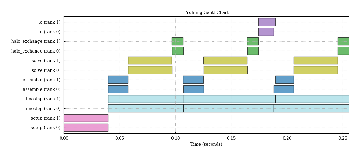
The chart displays one horizontal lane per (region, rank) combination, with bars spanning each recorded start-to-end interval. When multiple files are provided, each file gets its own stacked subplot in the exported chart.
Comparison bar charts from Python#
from scope_profiler import read_h5
from scope_profiler.plotting_scripts import plot_durations

runs = [
    read_h5("run_a.h5"),
    read_h5("run_b.h5"),
]

saved_paths = plot_durations(
    runs,
    filepath="durations.png",
    show=True,
)
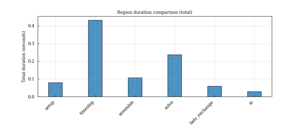
Each bar chart compares matching regions across files, with bars grouped
by file when several files are provided. plot_durations renders a
separate figure per requested statistic — by default avg, min,
max, and total duration per call. Use the metrics argument to
select a subset:
plot_durations(
    runs,
    metrics=["avg", "total"],
    filepath="durations.png",
    show=True,
)
When filepath is given and more than one metric is plotted, the metric
name is inserted before the file extension, e.g. durations_avg.png,
durations_total.png. plot_durations returns the list of filepaths it
wrote (empty if filepath is None).
Flame chart from Python#
from scope_profiler.plotting_scripts import plot_flame_chart

plot_flame_chart(results, ranks=[0], filepath="flame_chart.png", show=True)
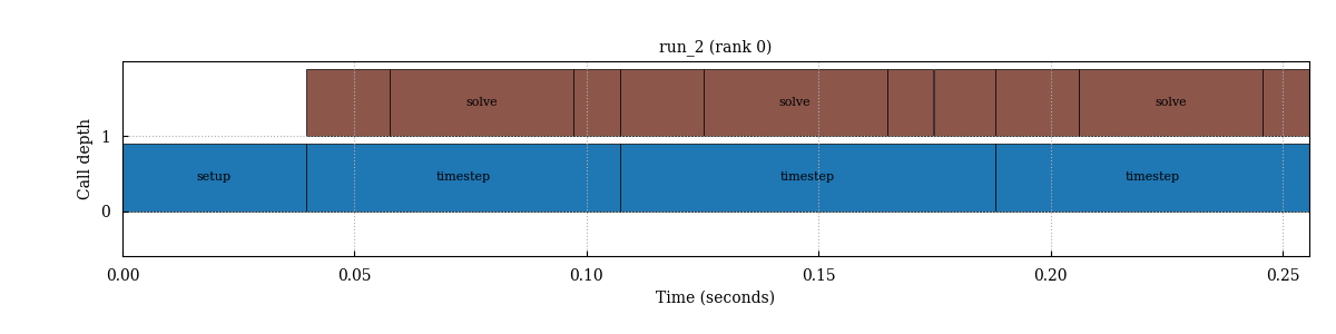
The call stack is reconstructed from timestamp containment: a region
whose interval falls inside another’s becomes its child. Unlike the
Gantt chart, the flame chart draws one panel per rank, defaulting to
rank 0 only, with time on the horizontal axis. The aggregated flame
graph is available as plot_flame_graph when the time axis is not
needed. Frame labels use the full reconstructed call path (for example,
timestep > assembly > solve), so same-named regions below different
parents remain distinguishable. Colors still identify the underlying
region. When source capture is enabled, the flame data export includes
each frame’s source_file and source_lineno; Plotly hover cards show
the same location.
Duration over time from Python#
from scope_profiler.plotting_scripts import plot_duration_timeseries

plot_duration_timeseries(results, filepath="duration_timeseries.png", show=True)
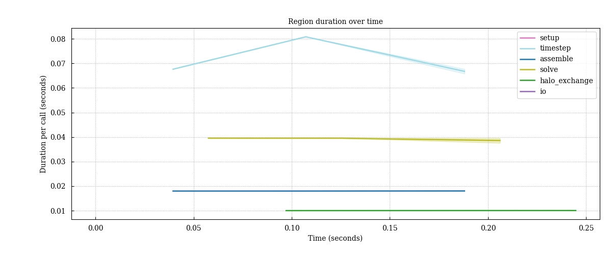
One line per region tracks the mean duration of each call over wall-clock time, shaded between the minimum and maximum across the selected ranks, so rank imbalance and drift over the run become visible.
Statistics JSON from Python#
from scope_profiler.plotting_scripts import (
    collect_region_statistics,
    write_region_statistics_json,
)

stats = collect_region_statistics(runs)                    # dict, nothing written
stats = write_region_statistics_json(runs, "stats.json")   # same dict, and a file
Both return per-file, per-region aggregates (count, average, min,
max, std, total, all in seconds), per-rank statistics for each
region, and the region names common to all inputs. This is the same
document scope-profiler plot default -o ... writes as
region_statistics.json.
Speedup graph from Python#
from scope_profiler import read_h5
from scope_profiler.plotting_scripts import plot_speedup

runs = [
    read_h5("run_1.h5"),
    read_h5("run_2.h5"),
    read_h5("run_4.h5"),
]

plot_speedup(
    runs,
    filepath="speedup.png",
    show=True,
)
The speedup plot shows one line per scope, with MPI rank count on the
x-axis and speedup on the y-axis, derived from average per-call
durations for each matching scope. The dashed reference line shows
optimal scaling relative to the smallest rank count present in the
inputs. x_field="num_nodes", "omp_num_threads" or "total_cores"
scales over nodes, threads, or ranks × threads instead.
create_html_report(runs, "scaling.html", speedup_x="nodes") sets the
x-axis of a comparison report’s speedup chart the same way: "auto"
(default), "ranks", "nodes", "threads" or "cores". A named axis
that some run did not record raises
scope_profiler.html_report.SpeedupAxisError (a ValueError).