Poisson's equation on nodes

Download notebook View on GitHubRun when the site was built.

NodalPoisson solves $-\nabla^2\phi = f$ with the unknowns on the cell corners. It suits codes whose own grid is node-centered, such as particle-in-cell codes that deposit charge on nodes: the base level of the hierarchy is their grid, and patches refine it where the field needs it. It takes Dirichlet and Neumann faces, periodic axes and electrodes inside the domain, and is factorized once, so that solving again costs two triangular solves.

import time

import numpy as np

from patchwork import (
    AMRHierarchy,
    Dirichlet,
    EmbeddedDirichlet,
    Neumann,
    NodalPoisson,
    plot_patches,
)

The mesh and its nodes

A patch of (nx, ny) cells has (nx + 1, ny + 1) nodes (Patch.node_shape). Patches that touch or nest share the nodes they have in common, so the solver numbers the nodes of the whole mesh once (solver.nodes). A node of a fine cell in the middle of a coarser cell’s edge is hanging: its value is interpolated between the ends of that edge, which keeps the potential continuous across patch boundaries. Here the y axis is periodic: its last node is its first.

mesh = AMRHierarchy(base_shape=(32, 32), periodic=(False, True))
mesh.add_patch(level=1, box=((24, 40), (24, 40)))
mesh.add_patch(level=2, box=((56, 72), (56, 72)))
fig, ax = plot_patches(mesh)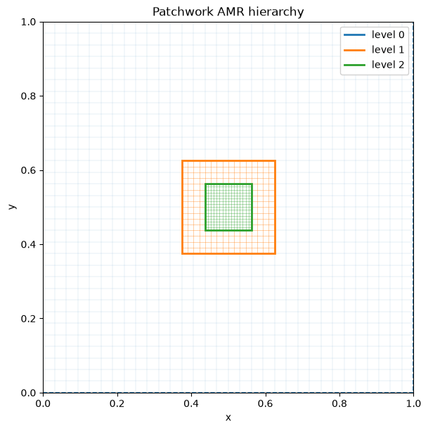

Conditions

Dirichlet(value) fixes the potential on a face, Neumann(gradient) its outward normal derivative. Both take a number or a function of x, y. A face that is not listed is grounded; the faces of a periodic axis take no condition.
EmbeddedDirichlet(inside, value) is an electrode at a fixed potential. inside tells which points it contains. Its surface is found by bisection along the mesh edges that enter it, and the nodes next to it use the distance to the surface (the Shortley-Weller stencil).

The problem needs at least one Dirichlet face or electrode; without one the potential is only known up to a constant, and the solver refuses it.

electrode = EmbeddedDirichlet(
    inside=lambda points: np.hypot(points[0] - 0.5, points[1] - 0.5) < 0.05,
    value=-20.0,
)
solver = NodalPoisson(
    mesh,
    faces={"x_lower": Neumann(0.0), "x_upper": Dirichlet(lambda x, y: 100.0 * y)},
    embedded=[electrode],
)
print(
    f"{solver.nodes.num_nodes} nodes, {solver.free.size} unknowns, "
    f"{int(solver.nodes.hanging.sum())} hanging nodes"
)

1472 nodes, 1247 unknowns, 64 hanging nodes

Solving, and solving again

The source and the result are arrays over solver.nodes; solver.nodes.coordinates gives the position of every node. With potential=... the result is also written to a node-centered field of the hierarchy, which plot_patches draws.

x, y = solver.nodes.coordinates.T
charge = 500.0 * np.exp(-((x - 0.3) ** 2 + (y - 0.5) ** 2) / 0.005)
potential = solver.solve(charge, potential="phi")
fig, ax = plot_patches(mesh, field="phi", show_grid=False)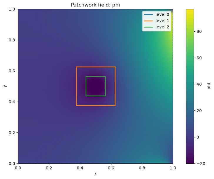

start = time.perf_counter()
for _ in range(100):
    solver.solve(charge)
print(f"{1e3 * (time.perf_counter() - start) / 100:.2f} ms per solve")

0.06 ms per solve

set_conditions changes face values and electrode potentials without factorizing again; a face keeps its kind (Dirichlet or Neumann).

solver.set_conditions(body_values=[+20.0])
flipped = solver.solve(charge)
on_electrode = electrode.inside(solver.nodes.coordinates.T)
print(
    f"potential on the electrode: {potential[on_electrode].mean():+.1f} V before, "
    f"{flipped[on_electrode].mean():+.1f} V after"
)

potential on the electrode: -20.0 V before, +20.0 V after

Patches where the field needs them

An electrode of half a base cell’s radius is more than the base mesh can resolve. Two nested patches around it bring the error down tenfold for a third more unknowns. The faces carry the exact potential of a disc at 1 V, so the error is known.

RADIUS = 0.03


def disc_potential(x, y):
    r = np.maximum(np.hypot(x - 0.5, y - 0.5), 1e-12)
    return np.where(r < RADIUS, 1.0, 1.0 + 0.5 * np.log(r / RADIUS))


disc = EmbeddedDirichlet(
    inside=lambda p: np.hypot(p[0] - 0.5, p[1] - 0.5) < RADIUS, value=1.0
)
faces = {
    face: Dirichlet(disc_potential)
    for face in ("x_lower", "x_upper", "y_lower", "y_upper")
}

for label, patches in (
    ("32 x 32 cells", []),
    ("with two nested patches", [(1, ((24, 40), (24, 40))), (2, ((56, 72), (56, 72)))]),
):
    mesh = AMRHierarchy(base_shape=(32, 32))
    for level, box in patches:
        mesh.add_patch(level=level, box=box)
    solver = NodalPoisson(mesh, faces=faces, embedded=[disc])
    nodes = solver.nodes
    result = solver.solve(np.zeros(nodes.num_nodes), potential="potential")
    on_base_nodes = np.all(nodes.lattice % nodes.cell_span.max() == 0, axis=1)
    error = np.abs(result - disc_potential(*nodes.coordinates.T))[on_base_nodes].max()
    print(f"{label:24s} {solver.free.size:5d} unknowns, error {error:.1e} V")

fig, ax = plot_patches(mesh, field="potential")
ax.set(xlim=(0.3, 0.7), ylim=(0.3, 0.7));

32 x 32 cells              960 unknowns, error 4.0e-02 V
with two nested patches   1268 unknowns, error 2.7e-03 V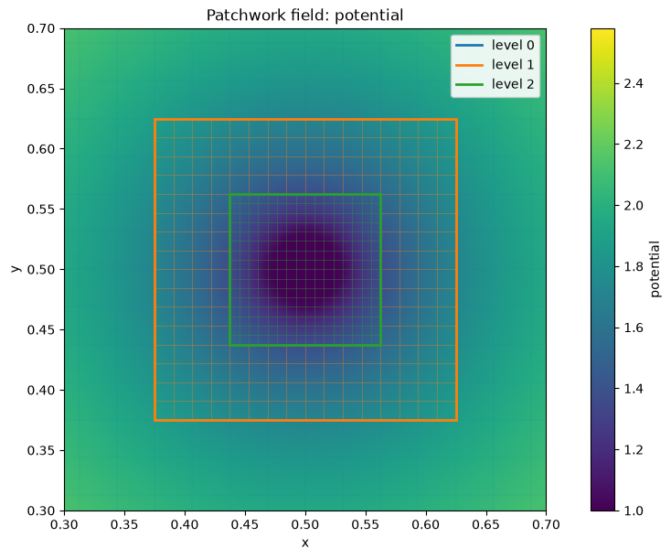

Hanging nodes are interpolated linearly, so across a patch boundary the error is that of the coarser side: put a patch boundary where the solution is smooth on the coarse mesh, a few cells away from the feature the patch resolves.

Fields on a uniform grid

A code that works on uniform arrays can move data in and out with the maps of solver.nodes:

from_level(0) interpolates values on the base grid to all nodes, e.g. a charge density deposited there;
to_level(level) samples the solution on the nodes of a level over the whole domain;
sample_patches(arrays, level) does the same for a field computed patch by patch, such as the gradient: each node takes the value of the finest patch around it.

base = nodes.level_shape(0)
uniform = (nodes.to_level(1) @ result).reshape(nodes.level_shape(1))
print("base lattice", base, "-> level-1 lattice", uniform.shape)
print("largest value on the level-1 lattice:", round(float(uniform.max()), 3))

base lattice (33, 33) -> level-1 lattice (65, 65)
largest value on the level-1 lattice: 2.58