A swarm in an electric field

Download notebook View on GitHubRun when the site was built.

In a swarm experiment, charged particles drift through a gas in a uniform field $E$ and reach a steady state where the energy gained from the field balances what collisions take away. ZeroDReactor does this with electric_field= and charges=: every step accelerates the charged species by $qE\,\Delta t/m$ and then collides them.

For a Maxwell-molecule cross section ( $\sigma = K/g$ , so the collision frequency $\nu = nK$ is constant) with isotropic elastic scattering, the steady state is known exactly. The drift velocity is

$v_d = \frac{qE}{\mu\nu}, \qquad \mu = \frac{mM}{m+M},$

and the mean energy follows Wannier’s relation

$\langle\varepsilon\rangle = \tfrac32 kT_g + \tfrac12 m v_d^2 + \tfrac12 M v_d^2 .$

Both check the field push and the collision kinematics together. For a real gas, compare the same diagnostics with a Boltzmann solver such as BOLSIG+ for the same cross-section set.

import numpy as np

import plasmacoll
from plasmacoll.constants import ATOMIC_MASS, BOLTZMANN, ELEMENTARY_CHARGE

m = M = 4.0026 * ATOMIC_MASS  # He+ drifting in He
mu = m * M / (m + M)
density, K, T_gas = 1e21, 1e-15, 300.0  # nu = n K = 1e6 /s
nu = density * K
gas = plasmacoll.NeutralBackground("He", density, T_gas, M)
elastic = plasmacoll.CollisionProcess(
    "elastic", "He", plasmacoll.CrossSection.maxwell_molecule(K, mu)
)


def swarm(field, seed=1):
    mcc = plasmacoll.MonteCarloCollisions(
        {"He+": m}, [gas], {"He+": [elastic]}, seed=seed
    )
    ions = plasmacoll.ParticleArrays.maxwellian(20_000, m, T_gas, seed=seed + 1)
    return plasmacoll.ZeroDReactor(
        mcc, {"He+": ions}, electric_field=(field, 0.0, 0.0), charges={"He+": 1}
    )

Approach to the steady state

At $E = 2$ kV/m the ions start thermal and accelerate until collisions balance the field, within a few collision times. Dashed lines are the steady-state values above.

dt = 0.02 / nu
field = 2e3
history = swarm(field).run(dt, 1000, every=10)
t = history.time * nu
v_d = ELEMENTARY_CHARGE * field / (mu * nu)
energy = (1.5 * BOLTZMANN * T_gas + 0.5 * (m + M) * v_d**2) / ELEMENTARY_CHARGE

fig, (left, right) = plt.subplots(1, 2, figsize=(9, 3.6))
left.plot(t, history.mean_velocity["He+"][:, 0] / 1e3, "o", ms=3, color=COLORS[0])
left.axhline(v_d / 1e3, ls="--", color=INK, label=r"$qE/(\mu\nu)$")
left.set(xlabel=r"$\nu t$", ylabel="drift velocity (km/s)", title="Drift velocity")
left.legend(frameon=False)
right.plot(t, history.mean_energy_ev["He+"], "o", ms=3, color=COLORS[1])
right.axhline(energy, ls="--", color=INK, label="Wannier")
right.set(xlabel=r"$\nu t$", ylabel="mean energy (eV)", title="Mean energy")
right.legend(frameon=False)
fig.tight_layout()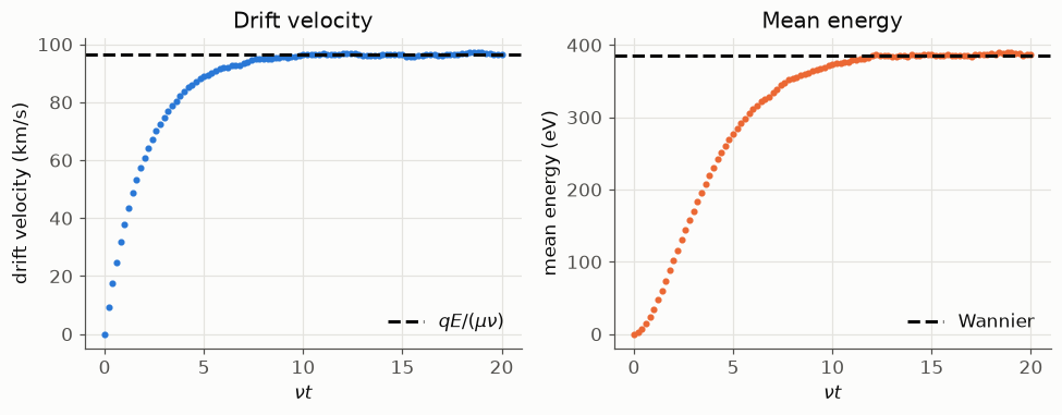

Mobility over a range of fields

The drift velocity is proportional to the field, and the mean energy grows with its square. Each point is the average over the steady state, from $\nu t = 10$ on.

fields = np.array([2e2, 5e2, 1e3, 2e3, 5e3])
drift, mean_energy = [], []
for index, field in enumerate(fields):
    history = swarm(field, seed=10 + index).run(dt, 1000, every=10)
    late = history.time * nu > 10
    drift.append(history.mean_velocity["He+"][late, 0].mean())
    mean_energy.append(history.mean_energy_ev["He+"][late].mean())
drift, mean_energy = np.array(drift), np.array(mean_energy)
expected_drift = ELEMENTARY_CHARGE * fields / (mu * nu)
expected_energy = (
    1.5 * BOLTZMANN * T_gas + 0.5 * (m + M) * expected_drift**2
) / ELEMENTARY_CHARGE

fig, (left, right) = plt.subplots(1, 2, figsize=(9, 3.6))
left.loglog(fields, drift, "o", color=COLORS[0], label="simulation")
left.loglog(fields, expected_drift, "--", color=INK, label=r"$qE/(\mu\nu)$")
left.set(xlabel="E (V/m)", ylabel="drift velocity (m/s)", title="Drift velocity")
left.legend(frameon=False)
right.loglog(fields, mean_energy, "o", color=COLORS[1], label="simulation")
right.loglog(fields, expected_energy, "--", color=INK, label="Wannier")
right.set(xlabel="E (V/m)", ylabel="mean energy (eV)", title="Mean energy")
right.legend(frameon=False)
for ax in (left, right):
    ax.minorticks_off()
    ax.set_xticks(fields, [f"{field:g}" for field in fields])
fig.tight_layout()
print(
    "largest relative error, drift :", np.abs(drift / expected_drift - 1).max().round(4)
)
print(
    "largest relative error, energy:",
    np.abs(mean_energy / expected_energy - 1).max().round(4),
)

largest relative error, drift : 0.0019
largest relative error, energy: 0.0087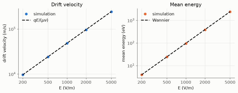

The simulation follows both laws to within about a percent over more than an order of magnitude in field. Where the ions’ energy approaches an inelastic threshold, add the inelastic processes and the drift velocity bends away from the straight line: that is where a comparison with measured mobilities or a Boltzmann solver starts to test the cross-section set itself.