Hydrogen and negative ions

Download notebook View on GitHubRun when the site was built.

Negative hydrogen ions are produced in the volume of a source by dissociative attachment of slow electrons to vibrationally excited hydrogen molecules.

The reaction is $e + \mathrm{H_2}(v) \to \mathrm{H^-} + \mathrm{H}$ , and its cross section rises by orders of magnitude from $v = 0$ to the highest levels. A collision model therefore needs the vibrational population, not just the H₂ density.

plasmacoll.vibrational provides a prescribed population: the measured H₂(X) vibrational ladder (Fantz and Wünderlich 2006) with one vibrational temperature. CrossSection.vibrational_mixture weights level-resolved cross sections with that population into a single attachment process. The level cross sections below are synthetic, because plasmacoll does not ship them. Replace them with tables from the literature.

import cunumpy as xp
import numpy as np

import plasmacoll
from plasmacoll.constants import ATOMIC_MASS, ELECTRON_MASS, ev_to_kelvin
from plasmacoll.vibrational import VibrationalDistribution

temperatures = (1000.0, 3000.0, 5000.0, 8000.0)
fig, ax = plt.subplots()
for color, temperature in zip(COLORS, temperatures, strict=False):
    distribution = VibrationalDistribution.h2_ground_state_from_kelvin(temperature)
    levels = np.arange(distribution.num_levels)
    ax.semilogy(
        levels,
        xp.to_numpy(distribution.populations),
        "o-",
        color=color,
        label=f"T_vib = {temperature:.0f} K",
    )
ax.set_ylim(1e-14, 1.5)
ax.set_xlabel("vibrational level v")
ax.set_ylabel("population n_v / n")
ax.set_title("Boltzmann populations of H₂(X, v)", loc="left")
ax.legend();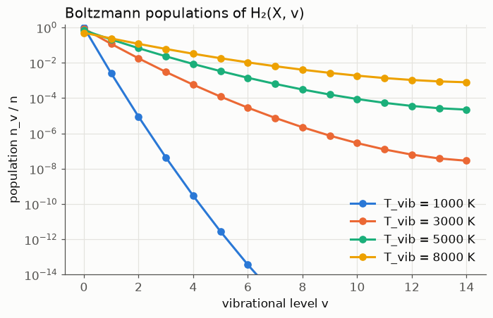

The excited fraction and an electronegativity estimate

$[\mathrm{H_2}(v\ge4)]/[\mathrm{H_2}]$ grows exponentially with $T_{vib}$ . estimate_electronegativity uses the balance of attachment against detachment by H atoms (Kimura and Kasugai 2010) to turn it into an order-of-magnitude $[\mathrm{H^-}]/[e]$ .

grid = np.linspace(1500, 9000, 60)
fractions = [
    VibrationalDistribution.h2_ground_state_from_kelvin(t).fraction_at_least(4)
    for t in grid
]
alpha = [
    plasmacoll.estimate_electronegativity(
        VibrationalDistribution.h2_ground_state_from_kelvin(t),
        hydrogen_atom_density=1e19,
        molecule_density=1e20,
    )
    for t in grid
]
fig, ax = plt.subplots()
ax.semilogy(grid, fractions, color=COLORS[0])
ax.set_xlabel("vibrational temperature (K)")
ax.set_ylabel("[H₂(v ≥ 4)] / [H₂]")
ax.set_title("Fraction of H₂ able to attach electrons efficiently", loc="left")
print(
    f"[H-]/[e] at 3000 K: {alpha[np.searchsorted(grid, 3000)]:.2e}, at 6000 K: {alpha[np.searchsorted(grid, 6000)]:.2e}"
)
plt.show()

[H-]/[e] at 3000 K: 7.79e-02, at 6000 K: 3.26e+00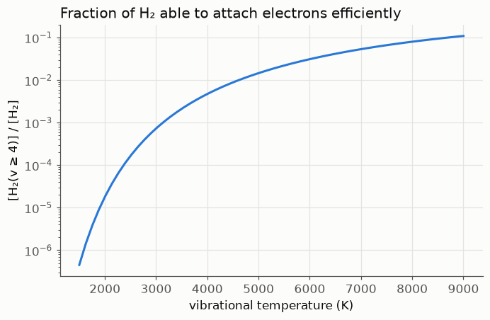

A population-weighted attachment process

Each synthetic level cross section is a resonance whose height grows tenfold every three levels. The mixture follows the vibrational temperature and goes into a single attachment process.

energy = np.linspace(0.0, 10.0, 201)


def synthetic_level(v):
    peak = max(0.3, 3.0 - 0.18 * v)
    return plasmacoll.CrossSection.from_function(
        lambda e: 1e-25 * 10 ** (v / 3) * np.exp(-0.5 * ((e - peak) / 0.8) ** 2),
        energy,
        label=f"synthetic v={v}",
    )


levels = [synthetic_level(v) for v in range(15)]
fig, ax = plt.subplots()
for color, temperature in zip(COLORS, temperatures, strict=False):
    distribution = VibrationalDistribution.h2_ground_state_from_kelvin(temperature)
    mixture = plasmacoll.CrossSection.vibrational_mixture(
        levels, distribution.populations
    )
    ax.semilogy(
        energy,
        xp.to_numpy(mixture(xp.asarray(energy))),
        color=color,
        label=f"T_vib = {temperature:.0f} K",
    )
ax.set_xlim(0, 6)
ax.set_ylim(1e-27, 1e-22)
ax.set_xlabel("electron energy (eV)")
ax.set_ylabel("cross section (m²)")
ax.set_title("Mixture of synthetic level cross sections", loc="left")
ax.legend();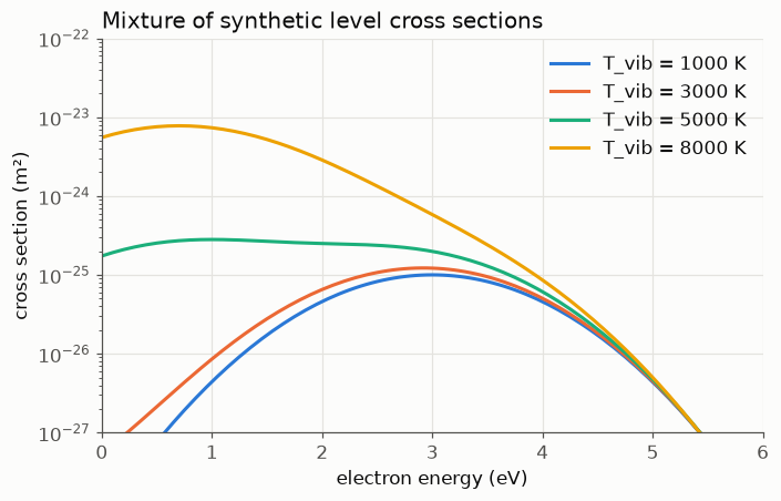

The rate coefficient $k = \langle\sigma v\rangle$ of electrons at $T_e = 1$ eV follows from the Maxwellian integral $k = \sqrt{8/(\pi m_e)}\,(kT_e)^{-3/2}\int \sigma(E)\,E\,e^{-E/kT_e}\,dE$ . A 0D reactor reproduces it from the counted attachments.

from plasmacoll.constants import ELEMENTARY_CHARGE

M_H2 = 2 * 1.008 * ATOMIC_MASS
T_e = 1.0  # eV
grid = np.linspace(1e-4, 30.0, 30_001)
n_gas, num, steps = 1e22, 200_000, 100

print("T_vib (K)   k from the integral   k from the reactor   attachments")
for temperature in temperatures:
    distribution = VibrationalDistribution.h2_ground_state_from_kelvin(temperature)
    mixture = plasmacoll.CrossSection.vibrational_mixture(
        levels, distribution.populations
    )
    sigma = xp.to_numpy(mixture(xp.asarray(grid)))
    integral = (
        np.trapezoid(sigma * grid * np.exp(-grid / T_e), grid) * ELEMENTARY_CHARGE**2
    )
    k_integral = (
        np.sqrt(8 / (np.pi * ELECTRON_MASS))
        * (T_e * ELEMENTARY_CHARGE) ** -1.5
        * integral
    )

    mcc = plasmacoll.MonteCarloCollisions(
        {"e": ELECTRON_MASS, "H-": M_H2 / 2},
        [plasmacoll.NeutralBackground("H2", n_gas, 500.0, M_H2)],
        {
            "e": [
                plasmacoll.CollisionProcess(
                    "attachment",
                    "H2",
                    mixture,
                    name="DA",
                    energy_frame="lab",
                    products={"negative_ion": "H-"},
                )
            ]
        },
        seed=1,
    )
    electrons = plasmacoll.ParticleArrays.maxwellian(
        num, ELECTRON_MASS, ev_to_kelvin(T_e), seed=2
    )
    # long enough for about 3 % of the electrons to attach: enough events, little depletion
    dt = 0.03 / (n_gas * k_integral * steps)
    history = plasmacoll.ZeroDReactor(mcc, {"e": electrons}).run(dt, steps, every=steps)
    attached = history.collisions["DA"][-1]
    k_reactor = -np.log(1 - attached / num) / (n_gas * steps * dt)
    print(
        f"{temperature:9.0f}   {k_integral:19.3e}   {k_reactor:18.3e}   {attached:11d}"
    )

T_vib (K)   k from the integral   k from the reactor   attachments
     1000             2.180e-20            2.129e-20          5777
     3000             2.874e-20            2.833e-20          5827
     5000             1.482e-19            1.480e-19          5905
     8000             2.728e-18            2.682e-18          5812