Getting started

Download notebook View on GitHubRun when the site was built.

Collide a population of electrons with a neutral gas: define cross sections, a background and the processes, build the operator, and look at the collision frequencies and the null-collision bound it collides with.

The cross sections here are simple model curves, chosen to show the machinery. They are not data for any real gas.

import cunumpy as xp
import numpy as np

import plasmacoll
from plasmacoll.constants import (
    ATOMIC_MASS,
    ELECTRON_MASS,
    ELEMENTARY_CHARGE,
    ev_to_kelvin,
)

Cross sections

A CrossSection is a table of cross section (m²) against energy (eV), interpolated linearly, constant beyond the last point and zero below the threshold. Tables come from text files (CrossSection.from_table), LXCat files (plasmacoll.read_lxcat), or functions sampled on a grid (CrossSection.from_function).

energy = np.geomspace(1e-2, 1e3, 400)

elastic = plasmacoll.CrossSection.from_function(
    lambda e: 8e-20 / (1 + (e / 10.0) ** 0.8), energy, label="elastic (model)"
)
excitation = plasmacoll.CrossSection.from_function(
    lambda e: 2e-21 * np.clip(e - 11.5, 0, None) / (1 + (e / 30.0) ** 1.5),
    energy,
    threshold=11.5,
    label="excitation (model)",
)
ionization = plasmacoll.CrossSection.from_function(
    lambda e: 3e-20 * np.log(np.clip(e / 15.8, 1, None)) / np.clip(e / 15.8, 1, None),
    energy,
    threshold=15.8,
    label="ionization (model)",
)

fig, ax = plt.subplots()
for table in (elastic, excitation, ionization):
    ax.loglog(
        xp.to_numpy(table.energy), xp.to_numpy(table(table.energy)), label=table.label
    )
ax.set_ylim(1e-22, 2e-19)
ax.set_xlabel("energy (eV)")
ax.set_ylabel("cross section (m²)")
ax.set_title("Model cross sections", loc="left")
ax.legend();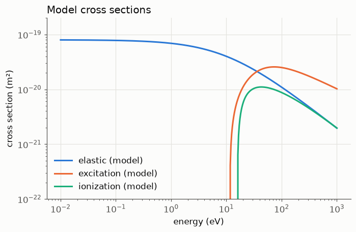

Background, processes and the operator

The neutral gas is a Maxwellian at rest with a density (m⁻³), a temperature (K) and a particle mass (kg). Each process names its kind, its background and its cross section; ionization also names the species of its products. The operator needs the mass of every species that collides or is created.

gas = plasmacoll.NeutralBackground(
    "gas", density=1e21, temperature=300.0, mass=40 * ATOMIC_MASS
)
products = {"electron": "e", "ion": "ion"}
mcc = plasmacoll.MonteCarloCollisions(
    species_masses={"e": ELECTRON_MASS, "ion": 40 * ATOMIC_MASS},
    backgrounds=[gas],
    processes={
        "e": [
            plasmacoll.CollisionProcess("elastic", "gas", elastic, energy_frame="lab"),
            plasmacoll.CollisionProcess(
                "excitation", "gas", excitation, energy_frame="lab"
            ),
            plasmacoll.CollisionProcess(
                "ionization", "gas", ionization, energy_frame="lab", products=products
            ),
        ]
    },
    seed=42,
)

Collision frequencies and the null-collision bound

Each step, every marker is a collision candidate with probability $1 - e^{-\nu_{\max}\,\Delta t}$ . A candidate then picks process $k$ with probability $\nu_k(g)/\nu_{\max}$ , or a null collision with the remaining probability. $\nu_{\max}$ has to bound the total frequency $\nu(g) = n\sum_k \sigma_k(E)\,g$ at every relative speed $g$ the markers can have. The operator tabulates the running maximum of $\nu(g)$ once, and takes the bound at the fastest marker of each step.

speeds = np.sqrt(2 * energy * ELEMENTARY_CHARGE / ELECTRON_MASS)
fig, ax = plt.subplots()
for process in mcc.processes["e"]:
    frequency = mcc.process_frequency("e", process, xp.asarray(speeds))
    ax.loglog(energy, xp.to_numpy(frequency), label=process.name)
total = xp.to_numpy(mcc.total_frequency("e", xp.asarray(speeds)))
bound = [mcc.frequency_bound("e", s) for s in speeds]
ax.loglog(energy, total, color=INK, label="total ν")
ax.loglog(energy, bound, color=INK, linestyle="--", label="bound ν_max")
ax.set_ylim(1e6, 3e10)
ax.set_xlabel("electron energy (eV)")
ax.set_ylabel("collision frequency (1/s)")
ax.set_title("Collision frequencies in a 10²¹ m⁻³ gas", loc="left")
ax.legend(loc="upper left");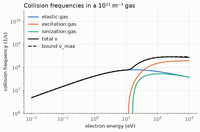

One collision step

collide works on plain arrays: positions (N, ndim), velocities (N, 3) in m/s and weights (N,). It returns the new velocities, a mask of the removed markers, the new markers per product species, and counters. Choose the time step so that $\nu_{\max}\Delta t \ll 1$ , since a marker collides at most once per step.

electrons = plasmacoll.ParticleArrays.maxwellian(
    100_000, ELECTRON_MASS, ev_to_kelvin(10.0), seed=1
)
nu_max = mcc.frequency_bound(
    "e", float(xp.max(xp.sqrt(xp.sum(electrons.velocities**2, axis=1))))
)
dt = 0.05 / nu_max
result = mcc.collide(
    "e", electrons.positions, electrons.velocities, electrons.weights, dt
)

d = result.diagnostics
print(f"nu_max dt = {nu_max * dt:.3f}")
print(f"candidates {d.candidates}, null {d.null_collisions}, real {d.real_collisions}")
for name, count in d.counts.items():
    print(f"  {name:22s} {count}")
print(
    "new markers:",
    {k: sum(len(b.weights) for b in v) for k, v in result.created.items()},
)

nu_max dt = 0.050
candidates 4913, null 3164, real 1749
  elastic:gas            1249
  excitation:gas         357
  ionization:gas         143
new markers: {'e': 143, 'ion': 143}

For a whole set of species, collide_species updates marker containers in place. It removes consumed markers and appends the products after all species have collided. ParticleArrays is one such container. A particle-in-cell code can pass its own containers through the MarkerSet protocol.