plasma-plots

What is plasma-plots?

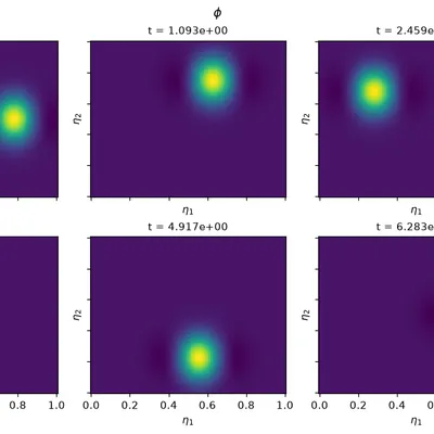
plasma-plots registers a .plasma accessor on xarray.DataArray and xarray.Dataset, and adds whole-run helpers for Struphy output, so you can go from a saved simulation to a figure in one line:

from struphy.post_processing.output import Output

out = Output("path/to/run")
out.evaluate("em_fields/phi").plasma.plot.slice(x="eta1", y="eta2", t=-1)

Loaded by Struphy

Creating a Struphy Output loads plasma-plots. For xarray data from elsewhere, import plasma_plots first; without it, .plasma raises AttributeError: 'DataArray' object has no attribute 'plasma'.

Output of other codes

plasma-plots reads labeled arrays, not Struphy files: arrays from any code work when their dimensions and coordinates follow the same names (t, eta1/eta2/eta3, X/Y/Z, marker). See Data from other codes.

Field plots

Time series, lineouts, 2-D slices, panels, vector fields, and animations — all driven by the labeled dimensions already on your output arrays.

Diagnostics

Growth/damping rate fits, envelopes, spatial averages, velocity moments, and dispersion relations via .plasma.analysis.

Whole-run overviews

Scalar energy histories and equilibrium profiles straight from a Struphy Output object.

3-D volumes

Optional PyVista integration for interactive 3-D volume rendering of scalar fields and equilibria.

Field lines & topology

Field lines traced through the mapped grid, Poincaré sections with island detection, connection lengths, O- and X-points and the reconnected flux.

A few examples

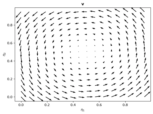
Vector field

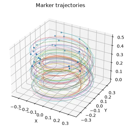
Marker trajectories

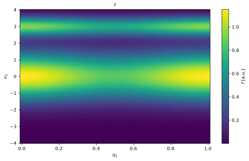
Phase-space distributions

3-D equilibrium views

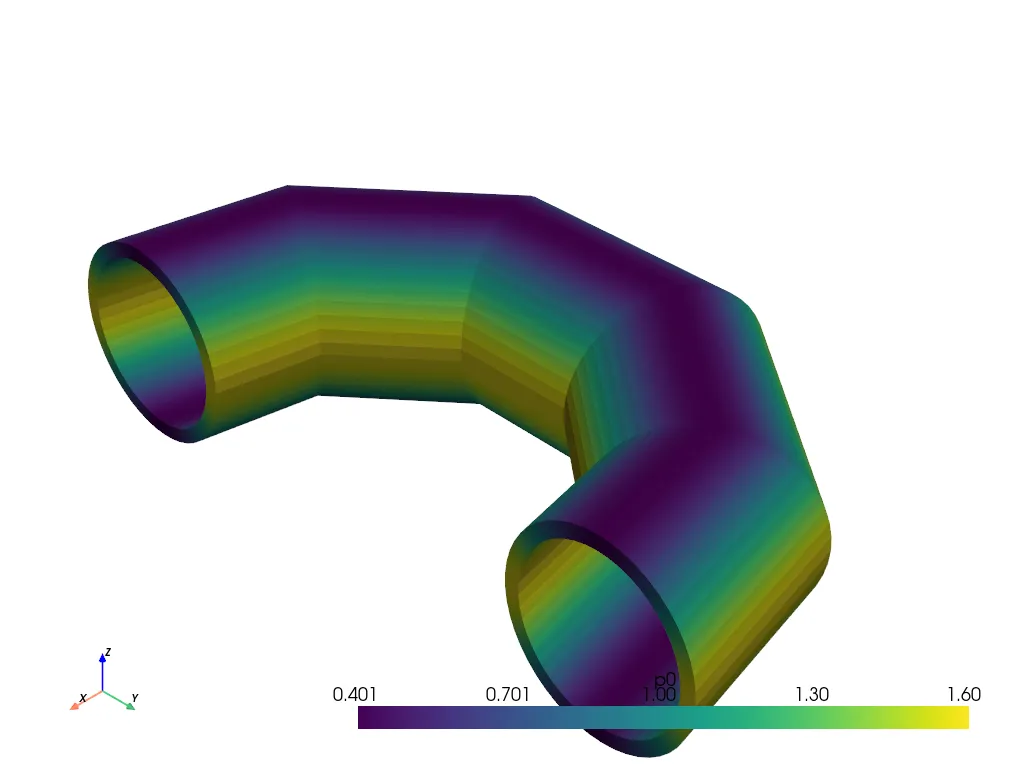
See Field plots, Time series & comparisons, Diagnostics, Particles & distributions, and Whole-run plots for the rest — every kind of plot and diagnostic plasma-plots has, with a real figure for each.

Looking for a simulation to plot?

plasma-plots plots data recorded by simulations such as Struphy’s; it doesn’t run any physics itself. If you want simulations to generate output from:

• Struphy’s examples gallery — Landau damping, the Orszag–Tang vortex, bump-on-tail, and dozens more, each with the model, domain, and parameters that produced it.
• MHD slab waves — every figure on that page comes from an actual Struphy run, reproduced by this repo’s own docs build.
• Struphy’s own documentation — models, propagators, domains, and everything else plasma-plots reads output from.