Ideal MHD test problems

Download notebookView on GitHubRun when the site was built.

Turbulence, Rotors, and Blast Waves in Magnetized Plasmas

Introduction

Magnetohydrodynamics (MHD) treats a plasma as a single conducting fluid threaded by a magnetic field. It governs everything from laboratory fusion devices and solar flares to galactic-scale dynamos. Understanding ideal MHD — without resistivity or viscosity — reveals the rich interplay between fluid motion and electromagnetic fields at its most fundamental level.

This tutorial runs three classic ideal MHD benchmark problems using the sandbox’s finite-volume IdealMHD2DSolver, each exposing a different facet of magnetized plasma dynamics:

Case	Phenomenon	Key physics
Orszag-Tang vortex	MHD turbulence	Magnetic reconnection, current sheets, energy cascade
MHD rotor	Field winding	Torsional Alfvén waves, angular momentum transport
Magnetized blast wave	Anisotropic shocks	Anisotropic fast-mode expansion, field compression

Setup

import matplotlib.colors as mcolors
import matplotlib.pyplot as plt
import numpy as np

from mhd_sandbox import Grid, IdealMHD2DSolver

CMAPS = {
    "density": "plasma",
    "pressure": "magma",
    "mag_pres": "cividis",
    "vorticity": "RdBu_r",
    "beta": "PuOr_r",
    "mach": "hot",
    "divB": "bwr",
}


def to_numpy(arr) -> np.ndarray:
    return arr.get() if hasattr(arr, "get") else np.asarray(arr)


def periodic_curl(vy, vx, dx, dy):
    dvydx = (np.roll(vy, -1, axis=0) - np.roll(vy, 1, axis=0)) / (2 * dx)
    dvxdy = (np.roll(vx, -1, axis=1) - np.roll(vx, 1, axis=1)) / (2 * dy)
    return dvydx - dvxdy


def compute_energies(solver):
    prims = solver.primitive_variables()
    rho, v, B, p = [
        to_numpy(prims[k])
        for k in ["density", "velocity", "magnetic_field", "pressure"]
    ]
    dV = solver.dx * solver.dy
    KE = 0.5 * np.sum(rho * np.sum(v**2, axis=-1)) * dV
    ME = 0.5 * np.sum(np.sum(B**2, axis=-1)) * dV
    TE = np.sum(p / (solver.gamma - 1)) * dV
    return float(KE), float(ME), float(TE)


def primitives_np(solver):
    return {k: to_numpy(v) for k, v in solver.primitive_variables().items()}


def grid_coords(solver):
    g = solver.grid
    nx, ny = g.num_gridpoints
    x = g.lower_bound[0] + (np.arange(nx) + 0.5) * solver.dx
    y = g.lower_bound[1] + (np.arange(ny) + 0.5) * solver.dy
    return x, y


def extent_from_solver(solver):
    g = solver.grid
    return g.lower_bound[0], g.upper_bound[0], g.lower_bound[1], g.upper_bound[1]


def plot_field_panel(ax, data, title, cmap, extent, symlog=False, label=""):
    if symlog:
        linthresh = max(1e-6, np.abs(data).max() * 0.01)
        norm = mcolors.SymLogNorm(linthresh=linthresh, vmin=data.min(), vmax=data.max())
    else:
        norm = mcolors.Normalize(vmin=data.min(), vmax=data.max())
    image = ax.imshow(
        data.T,
        origin="lower",
        extent=extent,
        cmap=cmap,
        norm=norm,
        aspect="equal",
    )
    ax.set_title(title, fontsize=10, fontweight="bold")
    ax.set_xlabel("x")
    ax.set_ylabel("y")
    ax.figure.colorbar(image, ax=ax, label=label)


def add_streamlines(ax, B, x, y, color="white", density=1.0):
    ax.streamplot(
        x,
        y,
        B[..., 0].T,
        B[..., 1].T,
        color=color,
        density=density,
        linewidth=0.5,
        arrowsize=0.5,
    )

Case 1 — Orszag-Tang Vortex

N_OT = 96
T_SNAPS = [0.0, 0.1, 0.2, 0.35, 0.5]
grid_ot = Grid(lower_bound=(0, 0), upper_bound=(1, 1), num_gridpoints=(N_OT, N_OT))
solver_ot = IdealMHD2DSolver(grid_ot, cfl=0.35)
solver_ot.set_state(IdealMHD2DSolver.orszag_tang_initial_state(grid_ot))
ot_snapshots, ot_energies = [], []


def _capture_ot():
    prims = primitives_np(solver_ot)
    B, v, p = prims["magnetic_field"], prims["velocity"], prims["pressure"]
    mag_p = 0.5 * np.sum(B**2, axis=-1)
    ot_snapshots.append(
        {
            "time": solver_ot.time,
            "rho": prims["density"],
            "p": p,
            "mag_p": mag_p,
            "vort": periodic_curl(v[..., 1], v[..., 0], solver_ot.dx, solver_ot.dy),
            "B": B,
            "beta": np.where(mag_p > 1e-12, p / mag_p, 50),
            "divB": to_numpy(solver_ot.divergence_b()),
        }
    )
    ot_energies.append(compute_energies(solver_ot))


_capture_ot()
for t in T_SNAPS[1:]:
    solver_ot.solve(t_end=t)
    _capture_ot()

fig, axes = plt.subplots(2, 4, figsize=(16, 7), layout="constrained")
fig.suptitle("Orszag-Tang Vortex — Evolution")
x_ot, y_ot = grid_coords(solver_ot)
ext_ot = extent_from_solver(solver_ot)
for col, idx in enumerate([0, 2, 3, 4]):
    s = ot_snapshots[idx]
    plot_field_panel(
        axes[0, col], s["rho"], f"Density t={s['time']:.2f}", CMAPS["density"], ext_ot
    )
    add_streamlines(axes[0, col], s["B"], x_ot, y_ot)
    plot_field_panel(
        axes[1, col], s["p"], f"Pressure t={s['time']:.2f}", CMAPS["pressure"], ext_ot
    )
plt.show()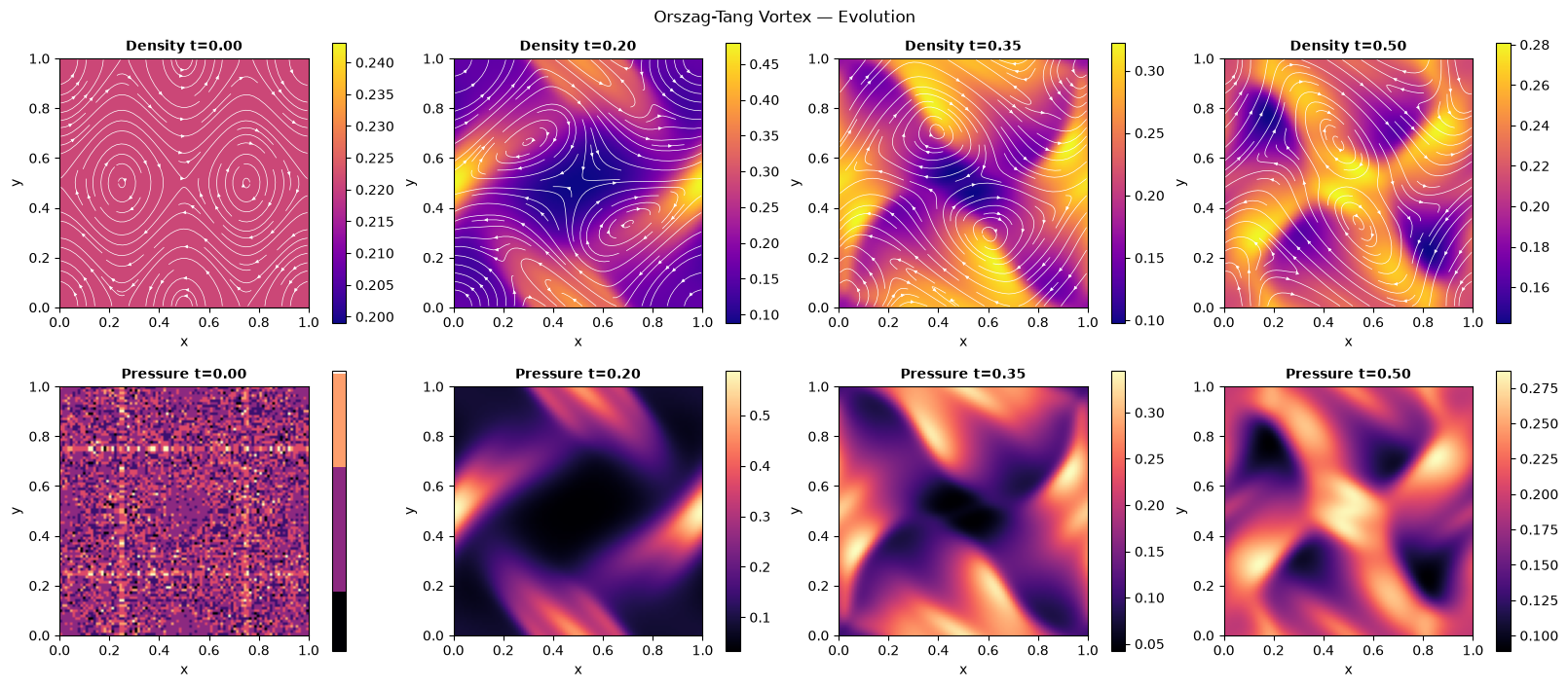

s = ot_snapshots[-1]
fig, axes = plt.subplots(2, 2, figsize=(9, 7.5), layout="constrained")
fig.suptitle(f"OT Vortex Diagnostics (t={s['time']:.2f})")
plot_field_panel(axes[0, 0], s["mag_p"], "Magnetic Pressure", CMAPS["mag_pres"], ext_ot)
add_streamlines(axes[0, 0], s["B"], x_ot, y_ot)
plot_field_panel(
    axes[0, 1], s["vort"], "Vorticity", CMAPS["vorticity"], ext_ot, symlog=True
)
plot_field_panel(
    axes[1, 0], np.clip(s["beta"], 0, 50), "Plasma Beta", CMAPS["beta"], ext_ot
)
plot_field_panel(
    axes[1, 1], s["divB"], "div(B) residual", CMAPS["divB"], ext_ot, symlog=True
)
plt.show()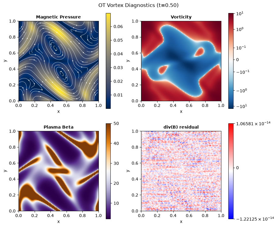

times_ot = [s["time"] for s in ot_snapshots]
KE, ME, TE = (
    np.array([e[0] for e in ot_energies]),
    np.array([e[1] for e in ot_energies]),
    np.array([e[2] for e in ot_energies]),
)
tot = KE + ME + TE
fig, ax = plt.subplots(figsize=(6, 4), layout="constrained")
ax.plot(times_ot, KE / tot[0], "C0-o", label="Kinetic")
ax.plot(times_ot, ME / tot[0], "C3-s", label="Magnetic")
ax.plot(times_ot, TE / tot[0], "C2-^", label="Thermal")
ax.plot(times_ot, tot / tot[0], "k--", label="Total")
ax.set_xlabel("Time")
ax.set_ylabel("Energy / E0")
ax.set_title("OT Energy Budget")
ax.legend()
plt.show()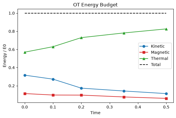

Case 2 — MHD Rotor

def make_rotor_ic(grid, v0=2.0, r0=0.1, r1=0.115):
    nx, ny = grid.num_gridpoints
    x0g, y0g = grid.lower_bound
    x1g, y1g = grid.upper_bound
    dx, dy = (x1g - x0g) / nx, (y1g - y0g) / ny
    x, y = x0g + (np.arange(nx) + 0.5) * dx, y0g + (np.arange(ny) + 0.5) * dy
    xx, yy = np.meshgrid(x, y, indexing="ij")
    r = np.sqrt((xx - 0.5) ** 2 + (yy - 0.5) ** 2)
    f = np.clip((r1 - r) / (r1 - r0), 0.0, 1.0)
    rho = np.where(r <= r0, 10.0, 1.0 + 9.0 * f * (r <= r1))
    rho = np.where(r > r1, 1.0, rho)
    vx = np.where(r <= r0, -v0 * (yy - 0.5) / r0, 0.0)
    vy = np.where(r <= r0, v0 * (xx - 0.5) / r0, 0.0)
    vx = np.where((r > r0) & (r < r1), -v0 * f * (yy - 0.5) / np.maximum(r, 1e-12), vx)
    vy = np.where((r > r0) & (r < r1), v0 * f * (xx - 0.5) / np.maximum(r, 1e-12), vy)
    v = np.zeros((nx, ny, 3))
    v[..., 0], v[..., 1] = vx, vy
    B = np.zeros((nx, ny, 3))
    B[..., 0] = 5.0 / np.sqrt(4.0 * np.pi)
    return IdealMHD2DSolver.primitive_to_conservative(rho, v, B, np.full((nx, ny), 1.0))


grid_rot = Grid(lower_bound=(0, 0), upper_bound=(1, 1), num_gridpoints=(96, 96))
solver_rot = IdealMHD2DSolver(grid_rot, cfl=0.3)
solver_rot.set_state(make_rotor_ic(grid_rot))
rot_snapshots = []


def _capture_rot():
    prims = primitives_np(solver_rot)
    B, v, rho = prims["magnetic_field"], prims["velocity"], prims["density"]
    v_mag = np.sqrt(np.sum(v**2, axis=-1))
    v_a = np.sqrt(np.sum(B**2, axis=-1) / np.maximum(rho, 1e-12))
    rot_snapshots.append(
        {
            "time": solver_rot.time,
            "rho": rho,
            "B": B,
            "v": v,
            "MA": v_mag / np.maximum(v_a, 1e-12),
            "mag_p": 0.5 * np.sum(B**2, axis=-1),
            "beta": np.where(
                np.sum(B**2, axis=-1) > 1e-12,
                prims["pressure"] / (0.5 * np.sum(B**2, axis=-1)),
                20,
            ),
        }
    )


_capture_rot()
for t in [0.05, 0.1, 0.15]:
    solver_rot.solve(t_end=t)
    _capture_rot()

fig, axes = plt.subplots(2, 4, figsize=(16, 7), layout="constrained")
fig.suptitle("MHD Rotor — Density & Alfvén Mach Evolution")
x_r, y_r = grid_coords(solver_rot)
ext_r = extent_from_solver(solver_rot)
for col, snap in enumerate(rot_snapshots):
    plot_field_panel(
        axes[0, col],
        snap["rho"],
        f"Density t={snap['time']:.2f}",
        CMAPS["density"],
        ext_r,
    )
    add_streamlines(axes[0, col], snap["B"], x_r, y_r)
    plot_field_panel(
        axes[1, col],
        np.clip(snap["MA"], 0, 5),
        f"MA t={snap['time']:.2f}",
        CMAPS["mach"],
        ext_r,
    )
    add_streamlines(axes[1, col], snap["B"], x_r, y_r, color="cyan", density=0.8)
plt.show()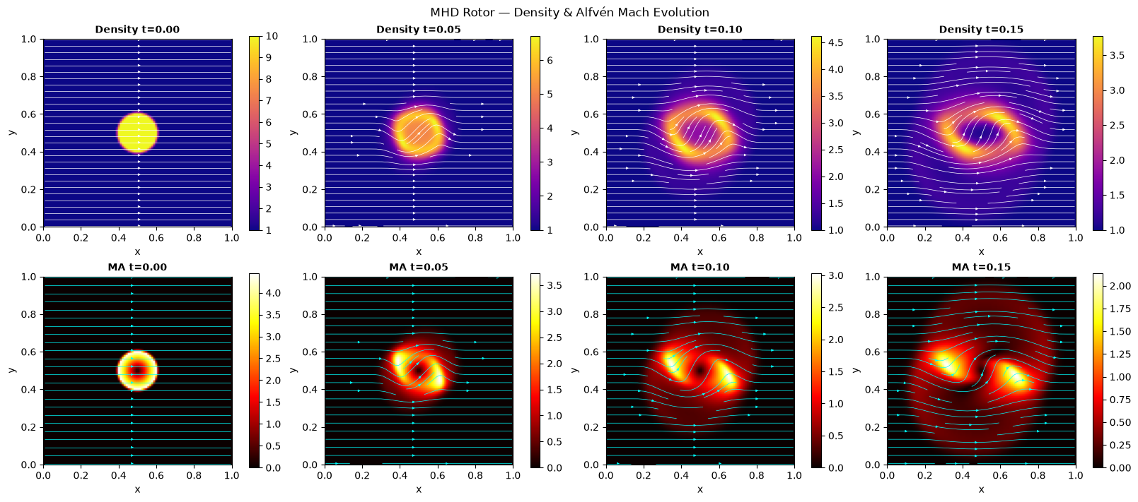

s = rot_snapshots[-1]
fig, axes = plt.subplots(1, 2, figsize=(10, 4.5), layout="constrained")
fig.suptitle(f"MHD Rotor Final State (t={s['time']:.2f})")
plot_field_panel(axes[0], s["mag_p"], "Magnetic Pressure", CMAPS["mag_pres"], ext_r)
add_streamlines(axes[0], s["B"], x_r, y_r, density=1.2)
plot_field_panel(
    axes[1], np.clip(s["beta"], 0, 20), "Plasma Beta", CMAPS["beta"], ext_r
)
add_streamlines(axes[1], s["B"], x_r, y_r, color="k", density=1.2)
plt.show()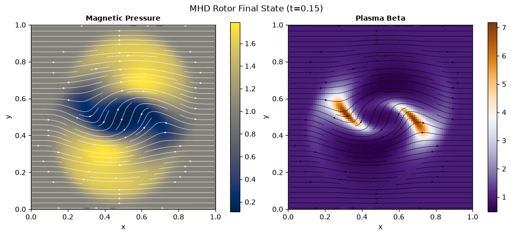

x_1d, y_1d = grid_coords(solver_rot)
XX, YY = np.meshgrid(x_1d, y_1d, indexing="ij")


def ang_mom(s):
    v = s["v"]
    L = s["rho"] * ((XX - 0.5) * v[..., 1] - (YY - 0.5) * v[..., 0])
    return float(np.sum(L) * solver_rot.dx * solver_rot.dy)


L_arr = [ang_mom(s) for s in rot_snapshots]
t_arr = [s["time"] for s in rot_snapshots]
fig, axes = plt.subplots(1, 2, figsize=(11, 4.5), layout="constrained")
fig.suptitle("MHD Rotor — Angular Momentum Transport")
axes[0].plot(t_arr, L_arr, "C3-o", lw=2.5)
axes[0].axhline(L_arr[0], color="gray", ls="--", label="Initial L")
axes[0].set_xlabel("Time")
axes[0].set_ylabel("L")
axes[0].set_title("Total Angular Momentum")
r_bins = np.linspace(0, 0.3, 30)
r_c = 0.5 * (r_bins[:-1] + r_bins[1:])
for idx, lbl, clr in [(0, "t=0.00", "C0"), (-1, f"t={t_arr[-1]:.2f}", "C3")]:
    snap = rot_snapshots[idx]
    r_f = np.sqrt((XX - 0.5) ** 2 + (YY - 0.5) ** 2)
    v_th = -snap["v"][..., 0] * (YY - 0.5) / np.maximum(r_f, 1e-12) + snap["v"][
        ..., 1
    ] * (XX - 0.5) / np.maximum(r_f, 1e-12)
    prof = [
        np.mean(v_th[(r_f >= r_bins[i]) & (r_f < r_bins[i + 1])])
        for i in range(len(r_bins) - 1)
    ]
    axes[1].plot(r_c, prof, lw=2, label=lbl, color=clr)
axes[1].axvline(0.1, color="gray", ls=":", label="Edge r0")
axes[1].set_xlabel("Radius r")
axes[1].set_ylabel("v_theta")
axes[1].set_title("Azimuthal Velocity Profile")
axes[1].legend()
plt.show()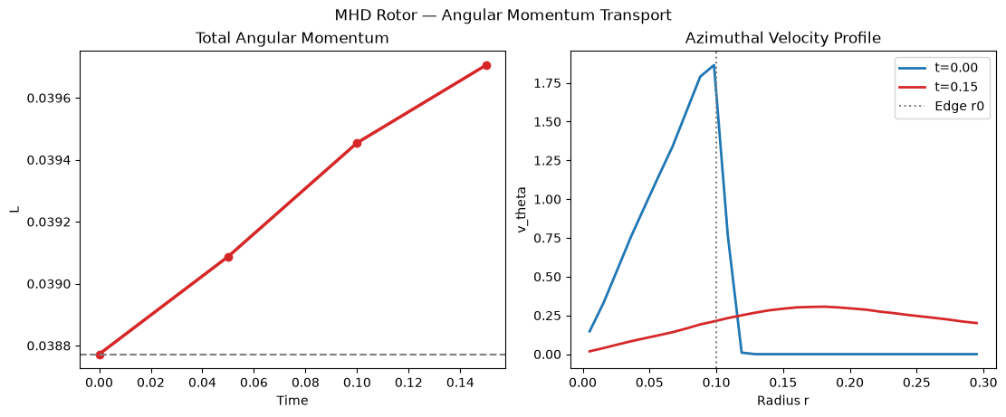

Case 3 — Magnetized Blast Wave

def make_blast_ic(grid, p_c=10.0, p_a=0.1, r_b=0.1, B0=1.0 / 2.0**0.5):
    nx, ny = grid.num_gridpoints
    x, y = np.linspace(0, 1, nx), np.linspace(0, 1, ny)
    xx, yy = np.meshgrid(x, y, indexing="ij")
    r = np.sqrt((xx - 0.5) ** 2 + (yy - 0.5) ** 2)
    rho = np.full((nx, ny), 1.0)
    p = np.where(r < r_b, p_c, p_a)
    B = np.zeros((nx, ny, 3))
    B[..., 0], B[..., 1] = B0, B0
    return IdealMHD2DSolver.primitive_to_conservative(rho, np.zeros((nx, ny, 3)), B, p)


grid_bl = Grid(lower_bound=(0, 0), upper_bound=(1, 1), num_gridpoints=(96, 96))
solver_bl = IdealMHD2DSolver(grid_bl, cfl=0.3)
solver_bl.set_state(make_blast_ic(grid_bl))
bl_snapshots = []


def _capture_bl():
    prims = primitives_np(solver_bl)
    rho, p, B, v = (
        prims["density"],
        prims["pressure"],
        prims["magnetic_field"],
        prims["velocity"],
    )
    cf = np.sqrt(solver_bl.gamma * p / rho + np.sum(B**2, axis=-1) / rho)
    bl_snapshots.append(
        {
            "time": solver_bl.time,
            "rho": rho,
            "p": p,
            "B": B,
            "MF": np.sqrt(np.sum(v**2, axis=-1)) / cf,
            "mag_p": 0.5 * np.sum(B**2, axis=-1),
        }
    )


_capture_bl()
for t in [0.05, 0.1, 0.2]:
    solver_bl.solve(t_end=t)
    _capture_bl()

fig, axes = plt.subplots(2, 4, figsize=(16, 7), layout="constrained")
fig.suptitle("Magnetized Blast Wave Evolution")
x_b, y_b = grid_coords(solver_bl)
ext_b = (0, 1, 0, 1)
for col, snap in enumerate(bl_snapshots):
    plot_field_panel(
        axes[0, col],
        snap["rho"],
        f"Density t={snap['time']:.2f}",
        CMAPS["density"],
        ext_b,
    )
    add_streamlines(axes[0, col], snap["B"], x_b, y_b)
    plot_field_panel(
        axes[1, col],
        snap["p"],
        f"Pressure t={snap['time']:.2f}",
        CMAPS["pressure"],
        ext_b,
    )
plt.show()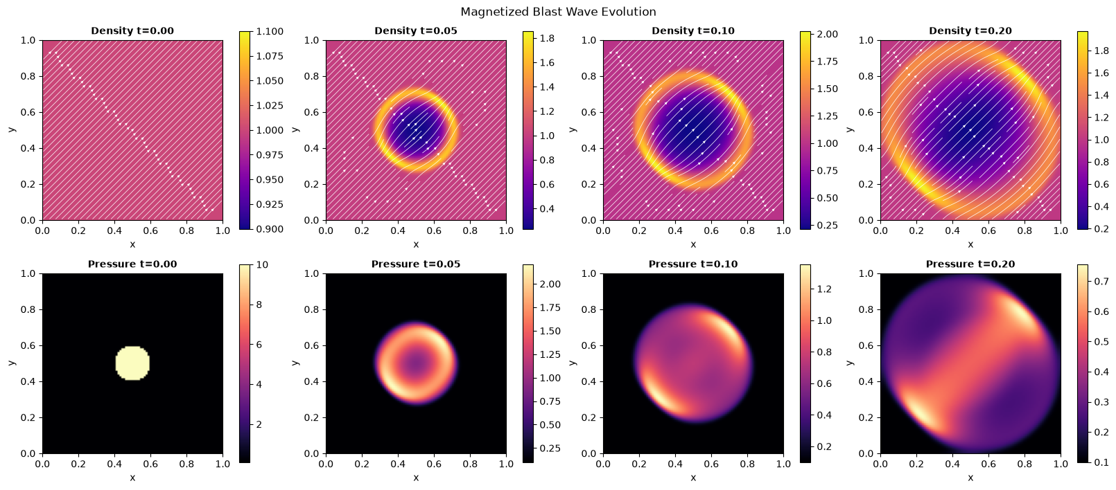

s = bl_snapshots[-1]
fig, axes = plt.subplots(1, 2, figsize=(10, 4.5), layout="constrained")
fig.suptitle(f"Blast Wave Final State (t={s['time']:.2f})")
plot_field_panel(axes[0], s["mag_p"], "Magnetic Pressure", CMAPS["mag_pres"], ext_b)
add_streamlines(axes[0], s["B"], x_b, y_b)
plot_field_panel(
    axes[1], np.clip(s["MF"], 0, 3), "Fast Mach Number", CMAPS["mach"], ext_b
)
add_streamlines(axes[1], s["B"], x_b, y_b, color="cyan", density=0.8)
plt.show()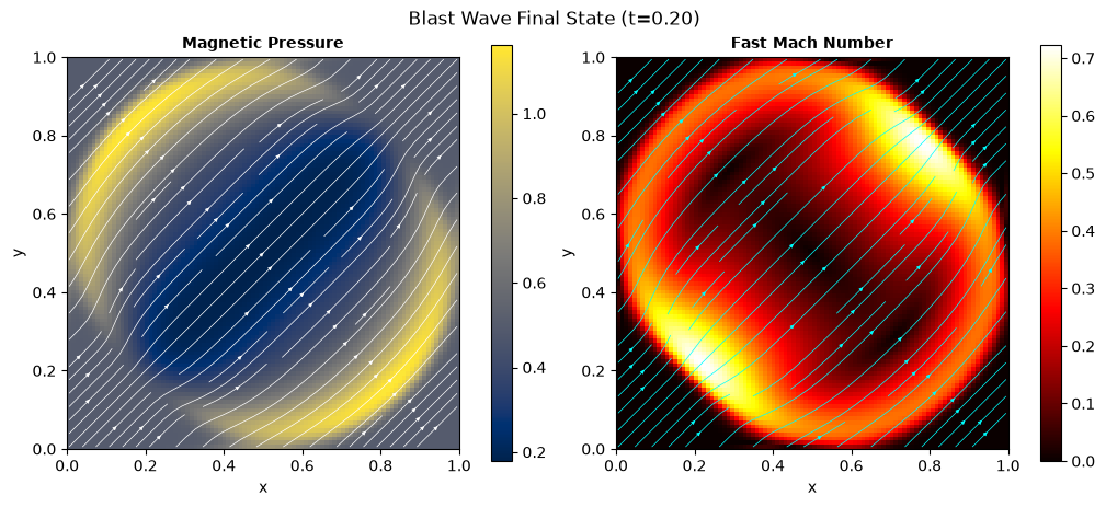

X_B, Y_B = np.meshgrid(x_b, y_b, indexing="ij")
r_f = np.sqrt((X_B - 0.5) ** 2 + (Y_B - 0.5) ** 2)
th_f = np.degrees(np.arctan2(Y_B - 0.5, X_B - 0.5))
r_bins = np.linspace(0, 0.48, 60)
r_c = 0.5 * (r_bins[:-1] + r_bins[1:])
fig, axes = plt.subplots(1, 2, figsize=(11, 4.5), layout="constrained")
fig.suptitle("Blast Wave Radial Profiles")
for c, (fn, yl) in enumerate([("rho", "Density"), ("p", "Pressure")]):
    data = bl_snapshots[-1][fn]
    masks = [
        (np.ones_like(th_f, dtype=bool), "Azimuthal avg", "C0", "-"),
        (np.abs(np.cos(np.radians(th_f + 45))) > 0.87, "Perp to B", "C2", "--"),
        (np.abs(np.cos(np.radians(th_f - 45))) > 0.87, "Para to B", "C3", "-."),
    ]
    for mask, lbl, clr, ls in masks:
        prof = []
        for i in range(len(r_bins) - 1):
            in_bin = (r_f >= r_bins[i]) & (r_f < r_bins[i + 1]) & mask
            # the innermost bins are narrower than a cell and may hold none
            prof.append(data[in_bin].mean() if in_bin.any() else np.nan)
        axes[c].plot(r_c, prof, label=lbl, color=clr, ls=ls)
    axes[c].axvline(0.1, color="gray", ls=":", label="Blast r0")
    axes[c].set_xlabel("Radius r")
    axes[c].set_ylabel(yl)
    axes[c].legend()
plt.show()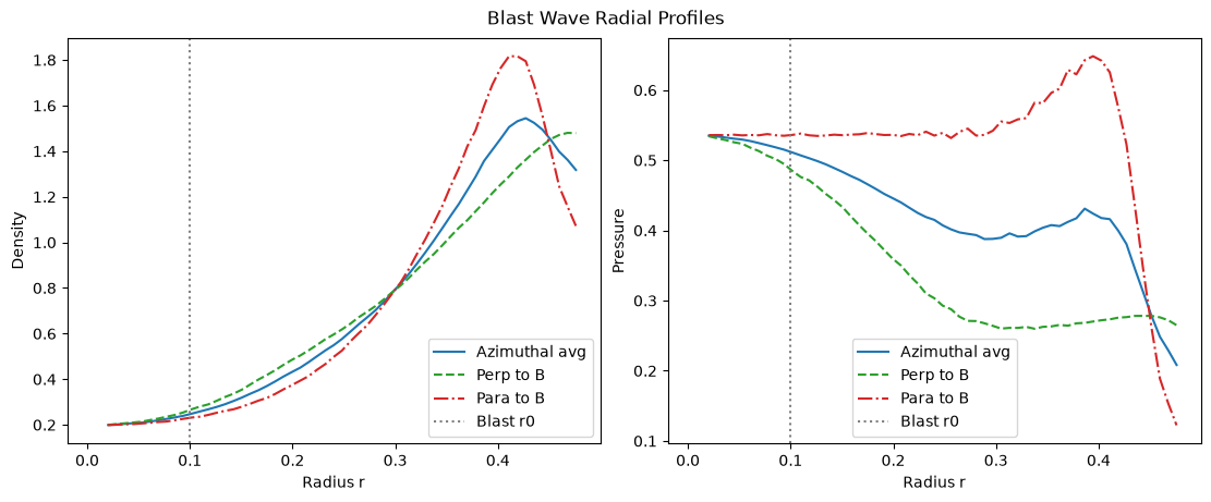

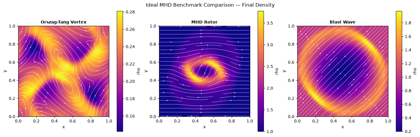
fig, axes = plt.subplots(1, 3, figsize=(14, 4.5), layout="constrained")
fig.suptitle("Ideal MHD Benchmark Comparison — Final Density")
for ax, (snap, solver, title) in zip(
    axes,
    [
        (ot_snapshots[-1], solver_ot, "Orszag-Tang Vortex"),
        (rot_snapshots[-1], solver_rot, "MHD Rotor"),
        (bl_snapshots[-1], solver_bl, "Blast Wave"),
    ],
    strict=True,
):
    ext = extent_from_solver(solver)
    xc, yc = grid_coords(solver)
    plot_field_panel(ax, snap["rho"], title, CMAPS["density"], ext, label="rho")
    add_streamlines(ax, snap["B"], xc, yc, density=0.8)
plt.show()