Multi-fluid ideal MHD
This tutorial runs two synchronized ideal-MHD fluids on a shared grid with MultiFluidIdealMHD2DSolver. Each fluid owns its conservative state and timestep constraint, while the multi-fluid wrapper advances all fluids with the most restrictive stable timestep. The setup below keeps the run small enough for documentation builds and compares a dense background fluid with a lighter beam-like fluid. The single-fluid reference problem is shown in the ideal MHD Orszag-Tang vortex tutorial.
import matplotlib.pyplot as pltimport numpy as np
from mhd_sandbox import Grid, MultiFluidIdealMHD2DSolver
grid = Grid(    lower_bound=(0.0, 0.0),    upper_bound=(1.0, 1.0),    num_gridpoints=(32, 32),)solver = MultiFluidIdealMHD2DSolver(    grid=grid,    fluid_names=["thermal_plasma", "beam_plasma"],    gammas={"thermal_plasma": 5.0 / 3.0, "beam_plasma": 1.4},    cfl=0.28,)
nx, ny = grid.num_gridpointsx = grid.lower_bound[0] + (np.arange(nx) + 0.5) * (    (grid.upper_bound[0] - grid.lower_bound[0]) / nx)y = grid.lower_bound[1] + (np.arange(ny) + 0.5) * (    (grid.upper_bound[1] - grid.lower_bound[1]) / ny)xx, yy = np.meshgrid(x, y, indexing="ij")
thermal_density = 1.0 + 0.12 * np.sin(2.0 * np.pi * xx) * np.sin(2.0 * np.pi * yy)thermal_velocity = np.zeros((nx, ny, 2))thermal_velocity[..., 0] = -0.25 * np.sin(2.0 * np.pi * yy)thermal_velocity[..., 1] = 0.25 * np.sin(2.0 * np.pi * xx)thermal_pressure = 0.8 + 0.04 * np.cos(2.0 * np.pi * xx)
beam_density = 0.35 + 0.18 * np.exp(-((xx - 0.28) ** 2 + (yy - 0.50) ** 2) / 0.025)beam_velocity = np.zeros((nx, ny, 2))beam_velocity[..., 0] = 0.55beam_velocity[..., 1] = 0.08 * np.sin(2.0 * np.pi * xx)beam_pressure = 0.28 + 0.02 * np.cos(2.0 * np.pi * yy)
magnetic_field = np.zeros((nx, ny, 2))magnetic_field[..., 0] = -np.sin(2.0 * np.pi * yy)magnetic_field[..., 1] = np.sin(4.0 * np.pi * xx)
solver.set_primitive(    "thermal_plasma",    thermal_density,    thermal_velocity,    magnetic_field,    thermal_pressure,)solver.set_primitive(    "beam_plasma", beam_density, beam_velocity, magnetic_field, beam_pressure)
Initial fluid states
Section titled “Initial fluid states”fig, axes = plt.subplots(1, 2, figsize=(10, 4.5), layout="constrained")for ax, data, title, cmap in [ (axes[0], thermal_density, "thermal_plasma density", "viridis"), (axes[1], beam_density, "beam_plasma density", "magma"),]: image = ax.imshow(data.T, origin="lower", extent=[0.0, 1.0, 0.0, 1.0], cmap=cmap) fig.colorbar(image, ax=ax) ax.set_xlim(0.0, 1.0) ax.set_ylim(0.0, 1.0) ax.set_title(title) ax.set_aspect("equal")plt.show()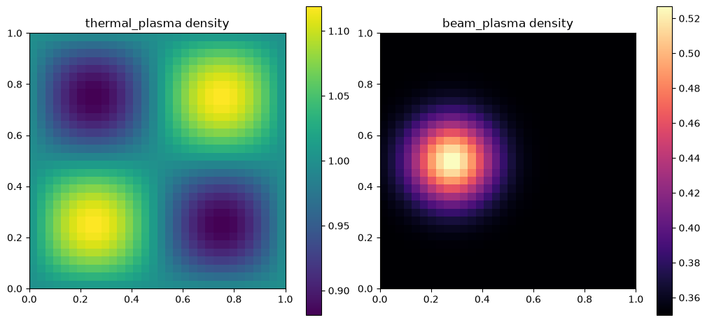
Advance both fluids with the shared timestep
Section titled “Advance both fluids with the shared timestep”time_history = [solver.time]thermal_mass = [float(np.sum(solver.primitive_variables("thermal_plasma")["density"]))]beam_mass = [float(np.sum(solver.primitive_variables("beam_plasma")["density"]))]max_divergence = [max(solver.max_abs_divergence_b().values())]
t_end = 0.015while solver.time < t_end: dt = min(solver.compute_dt(), t_end - solver.time) solver.step(dt) time_history.append(solver.time) thermal_mass.append( float(np.sum(solver.primitive_variables("thermal_plasma")["density"])) ) beam_mass.append( float(np.sum(solver.primitive_variables("beam_plasma")["density"])) ) max_divergence.append(max(solver.max_abs_divergence_b().values()))
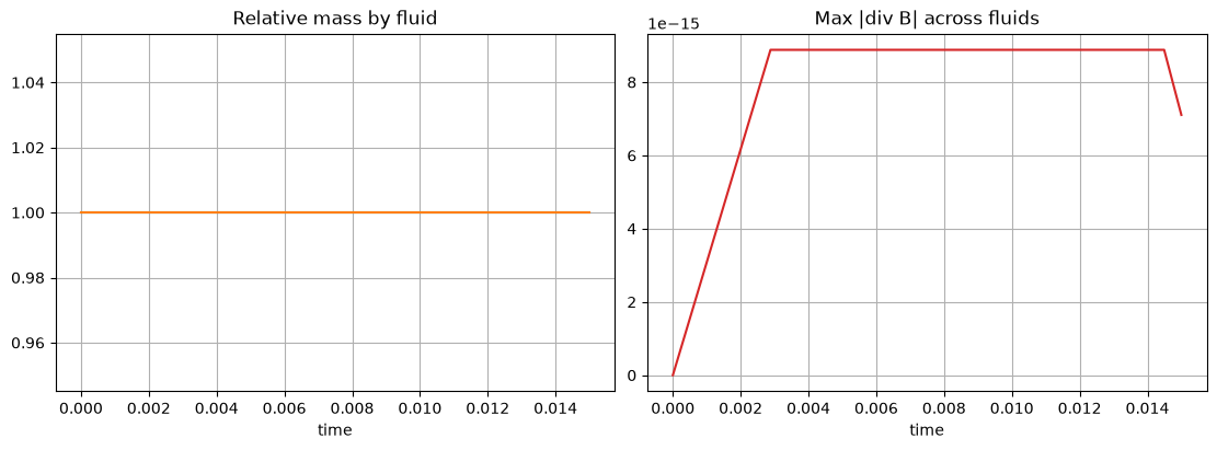
time_history = np.asarray(time_history)thermal_mass = np.asarray(thermal_mass)beam_mass = np.asarray(beam_mass)max_divergence = np.asarray(max_divergence)thermal = solver.primitive_variables("thermal_plasma")beam = solver.primitive_variables("beam_plasma")print(f"steps: {solver.steps}")print(f"time: {solver.time:.4f}")print(solver.max_abs_divergence_b())steps: 6time: 0.0150{'thermal_plasma': 7.105427357601002e-15, 'beam_plasma': 7.105427357601002e-15}fig, axes = plt.subplots(2, 2, figsize=(9, 8), layout="constrained")for ax, data, title, cmap in [ (axes[0, 0], thermal["density"], "thermal density", "viridis"), (axes[0, 1], beam["density"], "beam density", "magma"), (axes[1, 0], thermal["pressure"], "thermal pressure", "cividis"), (axes[1, 1], beam["pressure"], "beam pressure", "plasma"),]: image = ax.imshow(data.T, origin="lower", extent=[0.0, 1.0, 0.0, 1.0], cmap=cmap) fig.colorbar(image, ax=ax) ax.set_xlim(0.0, 1.0) ax.set_ylim(0.0, 1.0) ax.set_title(title) ax.set_aspect("equal")plt.show()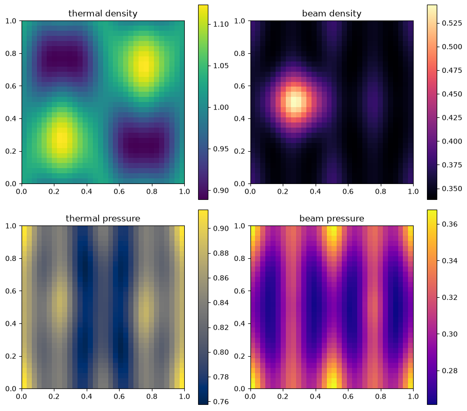
fig, axes = plt.subplots(1, 2, figsize=(11, 4), layout="constrained")axes[0].plot(time_history, thermal_mass / thermal_mass[0], color="tab:blue")axes[0].plot(time_history, beam_mass / beam_mass[0], color="tab:orange")axes[0].set_title("Relative mass by fluid")axes[0].set_xlabel("time")axes[0].grid(True)axes[1].plot(time_history, max_divergence, color="tab:red")axes[1].set_title("Max |div B| across fluids")axes[1].set_xlabel("time")axes[1].grid(True)plt.show()