Ideal MHD Orszag-Tang vortex
This example evolves the two-dimensional ideal MHD Orszag-Tang vortex and plots its density, pressure, magnetic pressure and vorticity.
Imports and helpers
Section titled “Imports and helpers”from __future__ import annotations
import matplotlib.pyplot as pltimport numpy as np
from mhd_sandbox import Grid, IdealMHD2DSolver
def _periodic_derivative(data: np.ndarray, spacing: float, axis: int) -> np.ndarray: """Return a centered periodic derivative.""" derivative = np.roll(data, shift=-1, axis=axis) derivative -= np.roll(data, shift=1, axis=axis) derivative /= 2.0 * spacing return derivativeParameters
Section titled “Parameters”num_gridpoints = (96, 96)t_end = 0.2show = FalseSet up and run the solver
Section titled “Set up and run the solver”grid = Grid( lower_bound=(0.0, 0.0), upper_bound=(1.0, 1.0), num_gridpoints=num_gridpoints,)
solver = IdealMHD2DSolver(grid=grid, cfl=0.3)solver.set_state(IdealMHD2DSolver.orszag_tang_initial_state(grid))result = solver.solve(t_end=t_end, verbose=True)MHD step 25, time=3.479753e-02, dt=1.361e-03, max|div B|=1.199e-14MHD step 50, time=6.810499e-02, dt=1.313e-03, max|div B|=1.066e-14MHD step 75, time=1.007620e-01, dt=1.307e-03, max|div B|=1.332e-14MHD step 100, time=1.338115e-01, dt=1.342e-03, max|div B|=1.332e-14MHD step 125, time=1.682095e-01, dt=1.395e-03, max|div B|=1.199e-14Derived fields
Section titled “Derived fields”primitives = solver.primitive_variables()density = primitives["density"]pressure = primitives["pressure"]velocity = primitives["velocity"]magnetic_field = primitives["magnetic_field"]
magnetic_pressure = 0.5 * np.sum(magnetic_field * magnetic_field, axis=-1)vorticity = _periodic_derivative(velocity[..., 1], solver.dx, axis=0)vorticity -= _periodic_derivative(velocity[..., 0], solver.dy, axis=1)Plot the fields
Section titled “Plot the fields”Each panel is a colour map with its colorbar; the magnetic field lines
are added with matplotlib’s streamplot.
fig, axes = plt.subplots(2, 2, figsize=(8.0, 6.8), layout="constrained")extent = [ grid.lower_bound[0], grid.upper_bound[0], grid.lower_bound[1], grid.upper_bound[1],]panels = [ (density, axes[0, 0], "Density", "magma"), (pressure, axes[0, 1], "Pressure", "viridis"), (magnetic_pressure, axes[1, 0], "Magnetic pressure", "cividis"), (vorticity, axes[1, 1], "Vorticity", "RdBu_r"),]for data, ax, title, cmap in panels: image = ax.imshow(data.T, origin="lower", extent=extent, cmap=cmap) fig.colorbar(image, ax=ax, shrink=0.85) ax.set(title=title, xlabel="x", ylabel="y", aspect="equal")
nx, ny = grid.num_gridpointsx = grid.lower_bound[0] + (np.arange(nx) + 0.5) * solver.dxy = grid.lower_bound[1] + (np.arange(ny) + 0.5) * solver.dyaxes[1, 0].streamplot( x, y, magnetic_field[..., 0].T, magnetic_field[..., 1].T, color="white", density=1.15, linewidth=0.45, arrowsize=0.55,)
fig.suptitle( f"Ideal MHD Orszag-Tang vortex, t={result.time:.2f}, " f"steps={result.steps}, max|div B|={result.max_divergence_b:.2e}")plt.show()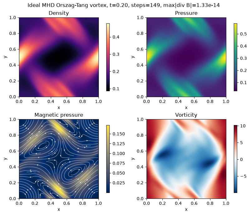
Inline animation
Section titled “Inline animation”import matplotlib.pyplot as pltimport numpy as npfrom IPython.display import HTML, displayfrom matplotlib import animation
from mhd_sandbox import Grid, IdealMHD2DSolver
def _periodic_derivative(data: np.ndarray, spacing: float, axis: int) -> np.ndarray: """Return a centered periodic derivative.""" derivative = np.roll(data, shift=-1, axis=axis) derivative -= np.roll(data, shift=1, axis=axis) derivative /= 2.0 * spacing return derivative
def _diagnostics(solver: IdealMHD2DSolver) -> dict[str, np.ndarray]: """Return scalar diagnostics for the current MHD state.""" primitives = solver.primitive_variables() velocity = primitives["velocity"] magnetic_field = primitives["magnetic_field"]
magnetic_pressure = 0.5 * np.sum(magnetic_field * magnetic_field, axis=-1) vorticity = _periodic_derivative(velocity[..., 1], solver.dx, axis=0) vorticity -= _periodic_derivative(velocity[..., 0], solver.dy, axis=1)
return { "density": primitives["density"], "pressure": primitives["pressure"], "magnetic_pressure": magnetic_pressure, "vorticity": vorticity, "magnetic_field": magnetic_field, }Parameters
Section titled “Parameters”num_gridpoints = (48, 48)t_end = 0.08num_frames = 12fps = 24grid = Grid( lower_bound=(0.0, 0.0), upper_bound=(1.0, 1.0), num_gridpoints=num_gridpoints,)solver = IdealMHD2DSolver(grid=grid, cfl=0.3)solver.set_state(IdealMHD2DSolver.orszag_tang_initial_state(grid))nx, ny = grid.num_gridpointsx = grid.lower_bound[0] + (np.arange(nx) + 0.5) * solver.dxy = grid.lower_bound[1] + (np.arange(ny) + 0.5) * solver.dyextent = [ grid.lower_bound[0], grid.upper_bound[0], grid.lower_bound[1], grid.upper_bound[1],]diagnostics = _diagnostics(solver)panels = [ ("density", "Density", "magma"), ("pressure", "Pressure", "viridis"), ("magnetic_pressure", "Magnetic pressure", "cividis"), ("vorticity", "Vorticity", "RdBu_r"),]fig, axes = plt.subplots(2, 2, figsize=(9.0, 7.2), layout="constrained")images = {}for ax, (key, title, cmap) in zip(axes.flat, panels, strict=True): images[key] = ax.imshow( diagnostics[key].T, origin="lower", extent=extent, cmap=cmap, interpolation="bilinear", ) ax.set_title(title) ax.set_xlabel("x") ax.set_ylabel("y") ax.set_aspect("equal") fig.colorbar(images[key], ax=ax, shrink=0.82, pad=0.02)quiver_stride = max(2, min(nx, ny) // 24)x_quiver = x[::quiver_stride]y_quiver = y[::quiver_stride]magnetic_field = diagnostics["magnetic_field"]magnetic_quiver = ax.quiver( x_quiver, y_quiver, magnetic_field[::quiver_stride, ::quiver_stride, 0].T, magnetic_field[::quiver_stride, ::quiver_stride, 1].T, color="white", pivot="mid", scale=24, width=0.003, alpha=0.9,)# Close the figure so only the animation below is displayed.plt.close(fig)Update plot
Section titled “Update plot”def update_plot(frame_index: int, target_time: float) -> None: """Advance the solver and update all plot artists.""" solver.solve(t_end=target_time) frame_diagnostics = _diagnostics(solver)
for key, _, _ in panels: data = frame_diagnostics[key] images[key].set_data(data.T) data_min = float(np.min(data)) data_max = float(np.max(data)) if data_min == data_max: padding = 0.5 if data_min == 0.0 else abs(data_min) * 0.05 data_min -= padding data_max += padding images[key].set_clim(data_min, data_max)
magnetic_field = frame_diagnostics["magnetic_field"] magnetic_quiver.set_UVC( magnetic_field[::quiver_stride, ::quiver_stride, 0].T, magnetic_field[::quiver_stride, ::quiver_stride, 1].T, )
fig.suptitle( f"Ideal MHD Orszag-Tang vortex " f"t={solver.time:.3f} step={solver.steps} " f"max|div B|={solver.max_abs_divergence_b():.1e}" ) print( f"frame {frame_index + 1:03d}/{num_frames}, " f"time={solver.time:.4f}, steps={solver.steps}" )output_times = np.linspace(0.0, t_end, num_frames)orszag_tang_animation = animation.FuncAnimation( fig, lambda frame_index: update_plot(frame_index, float(output_times[frame_index])), frames=num_frames, interval=1000 / fps, blit=False,)html = orszag_tang_animation.to_jshtml()display(HTML(html))frame 001/12, time=0.0000, steps=0frame 001/12, time=0.0000, steps=0frame 002/12, time=0.0073, steps=3frame 003/12, time=0.0145, steps=6frame 004/12, time=0.0218, steps=9frame 005/12, time=0.0291, steps=12frame 006/12, time=0.0364, steps=15frame 007/12, time=0.0436, steps=18frame 008/12, time=0.0509, steps=21frame 009/12, time=0.0582, steps=24frame 010/12, time=0.0655, steps=27frame 011/12, time=0.0727, steps=30frame 012/12, time=0.0800, steps=33