Two-stream instability
Two cold electron beams passing through each other bunch up and trap themselves in phase space.
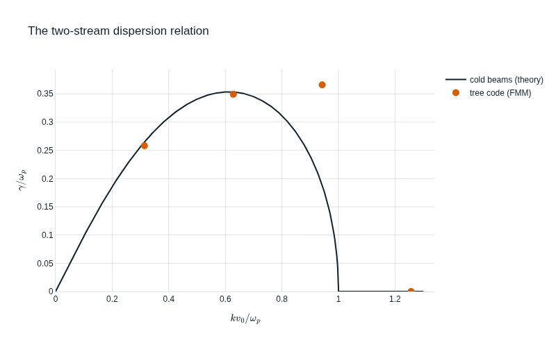
Two equal electron beams stream through each other at +v0 and -v0 across a fixed ion background that neutralises them. A small ripple of density along the beams is amplified: a beam slows where the potential is high and bunches there, which raises the potential further. For cold beams of plasma frequency omega_b = omega_p / sqrt(2) each, a mode k along the beams grows at gamma^2 = (sqrt(1 + 8 a^2) - 1 - 2 a^2) / 2 (in omega_p, with a = k v0 / omega_p) when a < 1, fastest, at gamma = omega_p / sqrt(8), for a^2 = 3/8. In a slab of plasma this holds for every bulk mode, whatever its shape across the slab. The growth stops when the beams’ electrons are trapped in the potential wells: the phase space (x, v_x) rolls up into vortices (electron holes), the textbook picture of a kinetic instability.
The plasma is a slab |y| < H/2, periodic along the beams (x, period L), with electrons and ions as line charges. A periodic sum of line charges is a free-space sum after the conformal map zeta = exp(2 pi i (x + i y) / L), which wraps the slab around an annulus: the field comes from the FMM of FlatQuadtree over the mapped charges (the system is neutral, so the map adds no field of its own), times d zeta / dz. The electrons are pushed with the leapfrog; the ions do not move. Units k_e = e = m_e = 1, omega_p = v0 = 1, L = 20 (modes k = 0.314 m), H = 5; the electrons start on the ion sites (a quiet start), displaced by a small ripple.
Source: examples/two_stream_instability.py. Run it yourself with python examples/two_stream_instability.py [--output examples/output] [--quick] (needs pip install "tree-d-3d[examples]").
Animations
Section titled “Animations”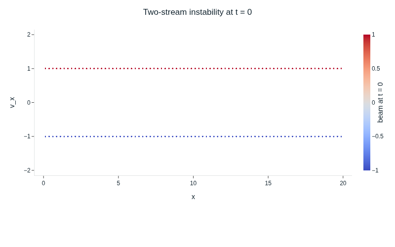
 Loading figure…
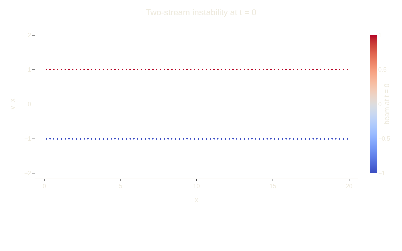
the electrons in (x, v_x), colored by their beam, as the most unstable mode (m = 2) grows, saturates and rolls the two beams up into two vortices (electron holes) of trapped electrons, which then slowly mix.
 Loading figure…
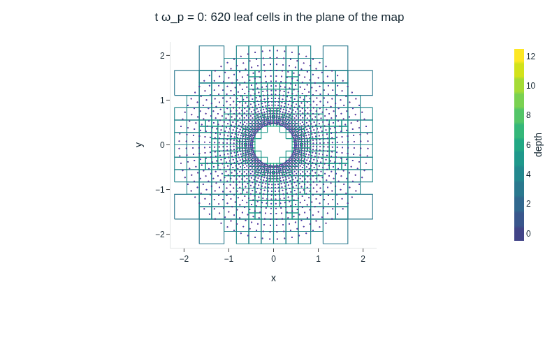
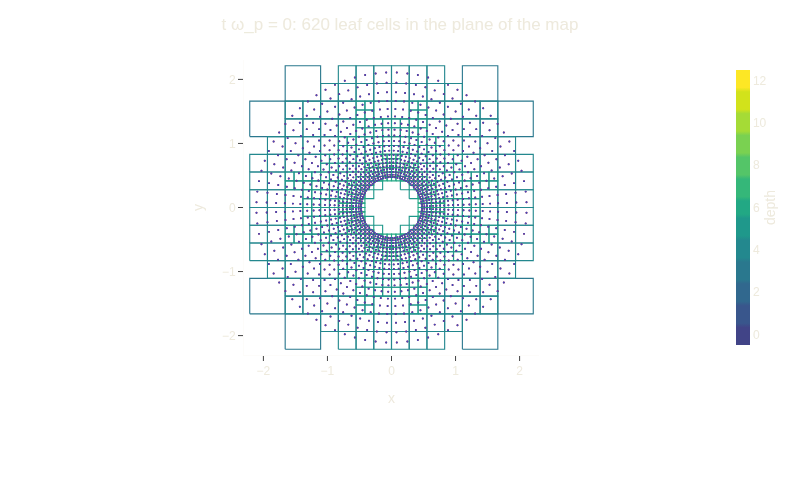
the same run in the plane of the map, with the quadtree the FMM builds every step: the slab is the annulus, the beams’ bunches are the spokes in which the cells crowd.
Figures
Section titled “Figures”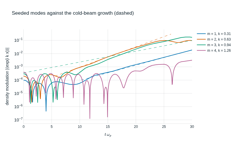
 Loading figure…
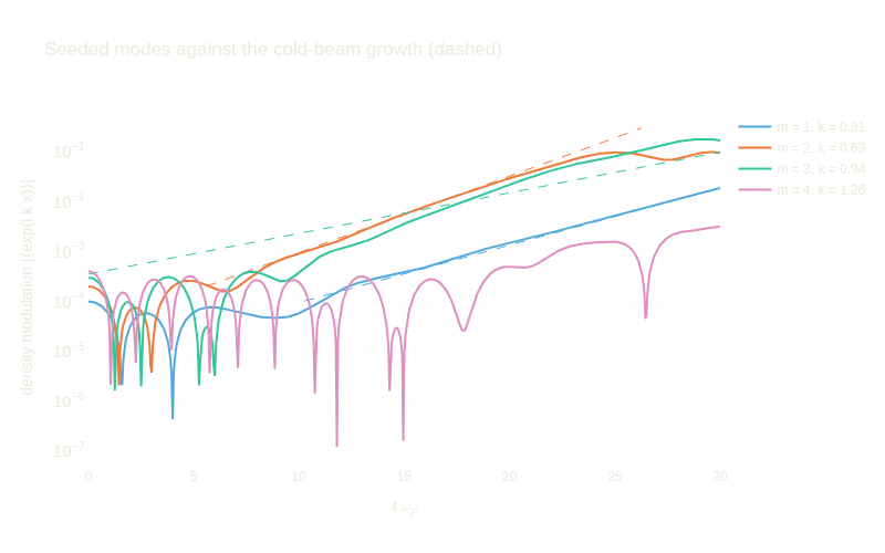
the density modulation of the seeded mode against time, one run per mode m = 1 ... 4, with the slope of the cold-beam growth rate (dashed); m = 4 (a = 1.26) is stable. Each run is seeded with the lowest bulk mode of the slab, the displacement grad(cos(k x) cos(pi y / H)), whose potential vanishes at the edges.
 Loading figure…
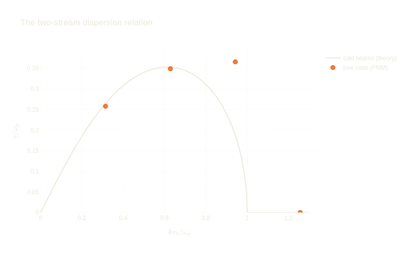
the growth rates fitted to the runs against the dispersion relation. m = 1, 2 and 4 agree with it; m = 3, near the cutoff, grows faster, at about the rate of m = 2: a mode of the edges of the slab, which the bulk theory leaves out. It weakens as the slab gets thicker (fitted 0.37, 0.29 and 0.26 at H = 5, 10 and 15, against 0.19 for the bulk). Usage::
--quick uses fewer electrons (about a minute); --smoke is the tiny configuration the test suite runs. Needs Plotly (pip install 'tree-d-3d[examples]').