Mesh-free beam optics
Steady-state space-charge optics without a mesh, with trajectories as line charges.
A steady beam is a bundle of trajectories; the trajectory carrying the current dI (per unit depth, in 2D) at speed v is a curve of line charge dI / v per unit length. Its space-charge field is then a sum over the charged segments of all trajectories, which the tree code evaluates in O(N) once the segments are turned into sources, and the self-consistent beam is the fixed point “trace in the field of the segments, rebuild the segments”. Mesh codes (IBSimu, picnic’s BeamOptics) deposit the trajectories on a grid and solve Poisson’s equation instead. This example runs the gridless loop on the one 2D case with an exact answer, a uniform sheet beam expanding under its own space charge: inside a uniform slab the field is linear in y, so the beam stays uniform and every trajectory follows y(x) = y0 (1 + kappa x^2) with kappa = q I / (4 eps0 m v0^3), the planar analogue of the envelope equation. Units q = m = eps0 = v0 = 1, half-width 1, I = 0.01 (kappa = 1/400, so the beam doubles in width over 20 units).
Each segment is represented by Gauss-Legendre points carrying its charge dI * dt, so no new kernel is needed; the segments of a trajectory are smoothed over a fraction of the trajectory spacing (the “ribbon”, a Plummer softening), which is what regularises the field a trajectory sees from itself and from its neighbours. A beam that starts and stops has fringe fields at its ends that the infinite slab does not (about a / (pi s) of the slab field at distance s from an end); mesh codes remove them with Neumann planes at the domain ends, and the gridless code does the same by mirroring the segments at x = 0 and x = L (images reflections on each side), which is exact for the self-similar beam at the entrance, where its mirror image is the converging beam.
Source: examples/segment_beam.py. Run it yourself with python examples/segment_beam.py [--output examples/output] [--quick] (needs pip install "tree-d-3d[examples]").
Figures
Section titled “Figures”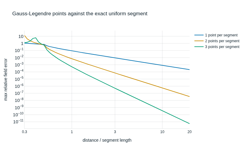
 Loading figure…
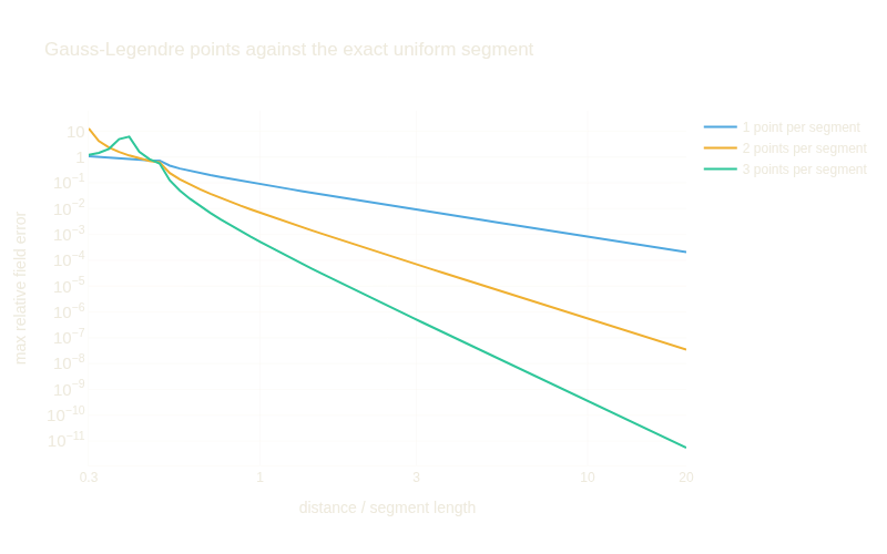
field error of 1, 2 and 3 Gauss-Legendre points per segment against the closed-form field of a uniform segment, against the distance over the segment length: the point representation is exponentially accurate beyond a segment length and only the near field needs the exact segment.
 Loading figure…
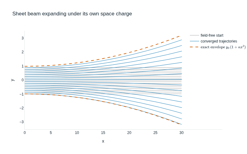
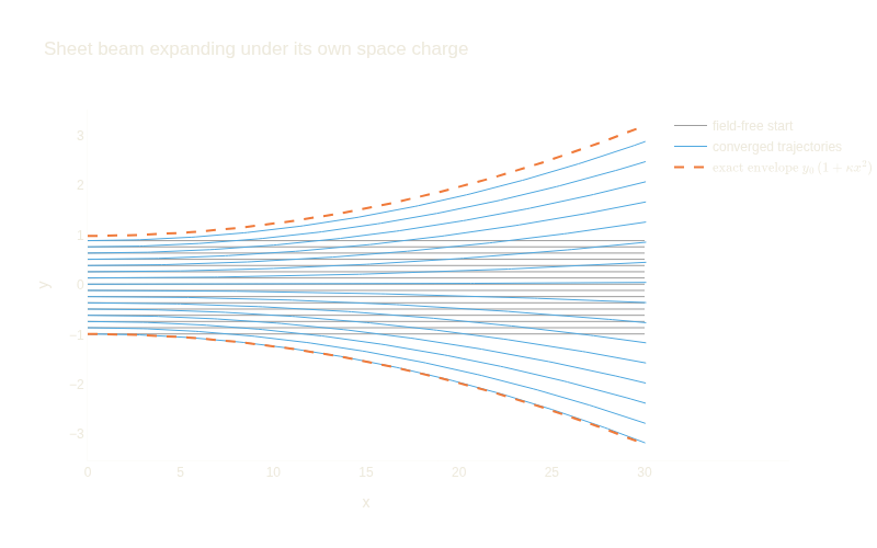
the converged trajectories, the envelope against the exact parabola, and the field-free straight rays the iteration starts from.
 Loading figure…
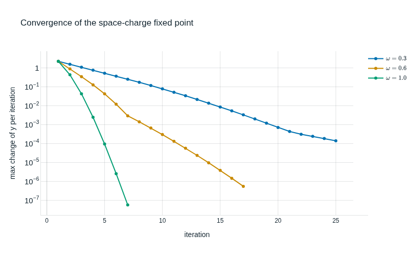
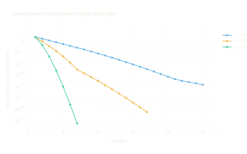
the change of the trajectories per iteration for several under-relaxation factors; for this beam plain substitution (omega = 1) converges fastest, and under-relaxation only slows it down.
 Loading figure…
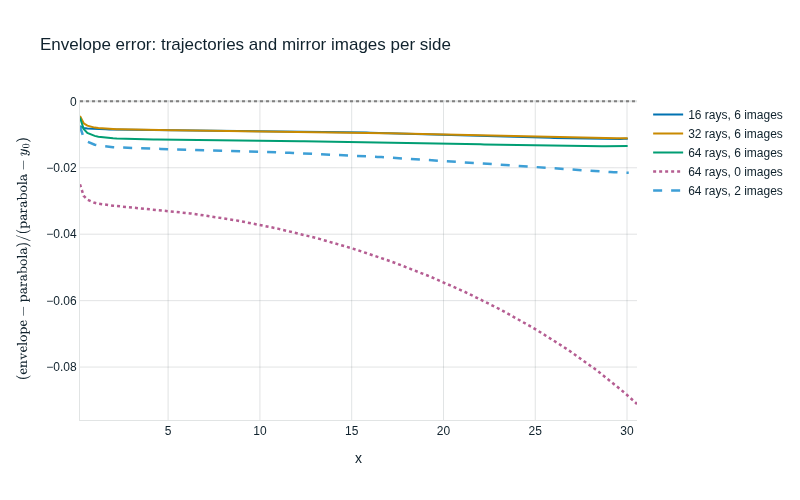
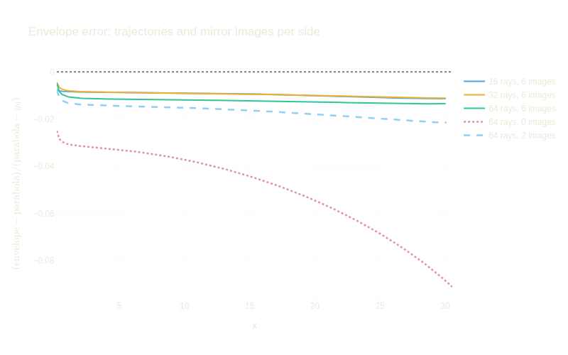
the envelope’s deviation from the parabola along the beam for several trajectory counts (ribbon width 0.3 spacings) and for several numbers of mirror images: the trajectory count hardly matters, the images do, because a mirrored beam is still finite and the missing far slabs at distance s cost about a / (pi s) of the field; the deviation falls as the images extend the beam.
 Loading figure…
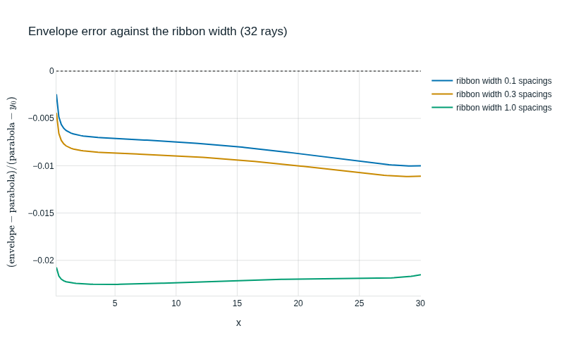
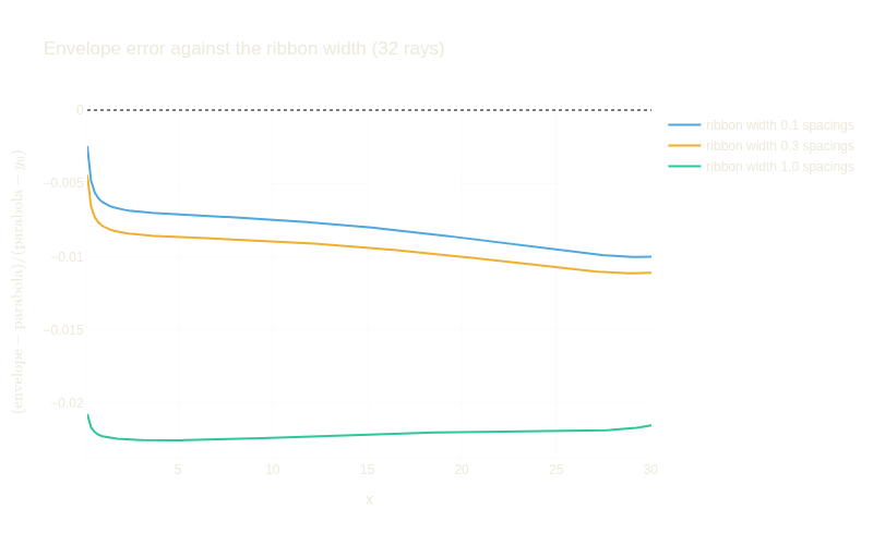
the same deviation against the ribbon width in trajectory spacings: a Plummer ribbon as wide as the spacing weakens the neighbours’ field (the softened field at one spacing is half the bare one, a deficit of about one trajectory’s worth in the whole slab), a narrow one leaves the discrete trajectories’ noise; the width is a numerical parameter of the method, as the cell size is for a mesh.
--quick uses fewer trajectories (a few minutes instead of ten); --smoke is the tiny configuration the test suite runs. Needs Plotly (pip install 'tree-d-3d[examples]').