Inspecting geometry

Download notebook View on GitHubRun when the site was built.

Explore 2D objects, named collections, grids and 3D surfaces with show(), plot() and show_3d(). All examples run without Picnic.

Install simgeometry[plot] for these examples. Plotting imports its dependencies only when used. Calls return Matplotlib axes that you can customize or save. show() displays a view; plot() draws without displaying. A 3D object defaults to a 3D view, while show(z=...) selects a section.

import matplotlib.pyplot as plt

from simgeometry import Circle, GeometryCollection, Grid, Rectangle, Sphere

geometry = GeometryCollection(
    {
        "electrode": Circle((0.25, 0.0), 0.35),
        "wall": Rectangle((-0.6, 0.0), (0.15, 1.3)),
    },
    bounds=((-1.0, -0.8), (1.0, 0.8)),
    styles={"electrode": {"color": "tab:orange"}, "wall": {"color": "tab:blue"}},
)
grid = Grid(
    ndim=2, lower_bound=(-1.0, -0.8), upper_bound=(1.0, 0.8), num_gridpoints=(25, 21)
)
ax = geometry.show(grid=grid, nodes=True, display=False)
ax.set_title("Objects, solid nodes, and grid lines")
plt.show()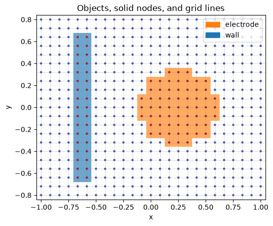

Compose views and save figures

Reuse an axes object when composing panels. A grid overlay samples membership at the grid nodes, so coarse grids look discrete. Without a grid, resolution controls the sampling used for display. Existing Shape2D.plot() continues to draw primitive polygon outlines.

ring = Circle((0, 0), 0.7) - Circle((0, 0), 0.3)
fig, axes = plt.subplots(1, 2, figsize=(9, 4), layout="constrained")
ring.plot(ax=axes[0], resolution=160, color="tab:green", labels=False)
axes[0].set_title("A ring: its hole stays empty")
geometry.plot(ax=axes[1], resolution=160)
axes[1].set_title("Named objects")
# fig.savefig("geometry.png", dpi=160)
plt.show()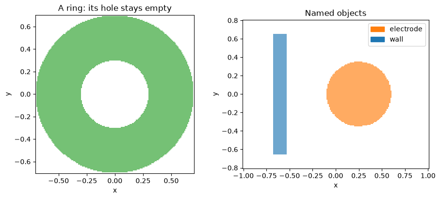

Three-dimensional inspection

The 3D view extracts a surface mesh. resolution controls its sampling; it does not alter the geometry’s containment queries. A static clipping plane retains the side toward its normal and leaves the cut open.

ball = Sphere((0, 0, 0), 1)
fig = plt.figure(figsize=(10, 4), layout="constrained")
ax = fig.add_subplot(121, projection="3d")
ball.show_3d(ax=ax, resolution=28, opacity=0.65, display=False, labels=False)
ax.set_title("Surface")
ax = fig.add_subplot(122, projection="3d")
ball.show_3d(
    ax=ax,
    resolution=28,
    clip=((0, 0, 0), (1, 0, 0)),
    normals=True,
    display=False,
    labels=False,
)
ax.set_title("Clipped surface and outward normals")
plt.show()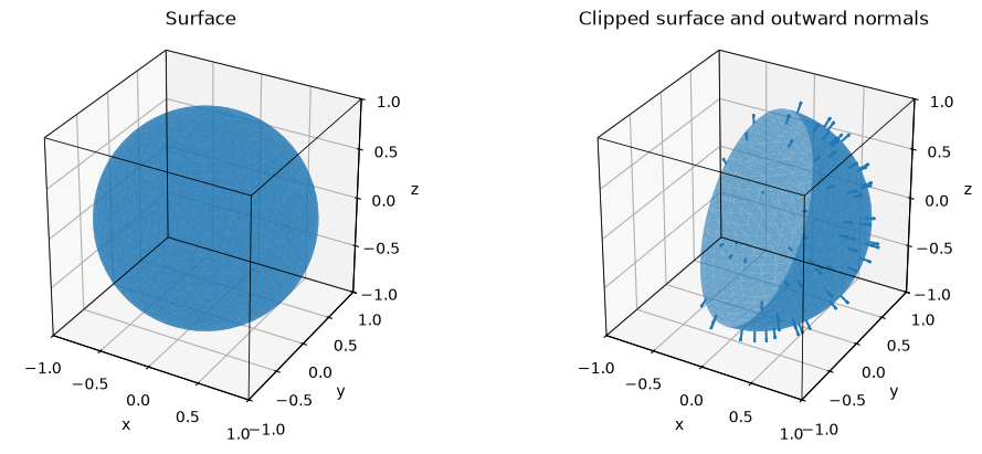

Interactive clipping

Install simgeometry[interactive] and run this locally to get an interactive clipping-plane widget:

viewer = ball.show_3d(backend="pyvista", clip=True, opacity=0.6)
viewer.close()  # release the viewer when finished

Matplotlib also supports rotating its 3D axes in an interactive window. For batch output, use display=False, save="geometry.png".

Try changing the sphere resolution from 16 to 64 and compare its silhouette. For a thin shell or a small hole, check that the feature survives refinement rather than trusting one picture.