Grid intersections and cut edges

Download notebook View on GitHubRun when the site was built.

Inspect the geometric input to a cut-cell solver: crossing positions, edge fractions, distances, object identity, and outward normals. Simgeometry computes geometry; Picnic applies its Shortley–Weller coefficients, boundary conditions and numerical minimum-distance clamp.

This notebook needs simgeometry[plot]. It does not solve a PDE. The companion Picnic cut-cell tutorial studies potential and electric-field accuracy.

import matplotlib.pyplot as plt
import numpy as np

from simgeometry import Circle, GeometryCollection, Grid
from simgeometry.cut_edges import bracketed_edge_geometry

grid = Grid(ndim=2, lower_bound=(-1, -1), upper_bound=(1, 1), num_gridpoints=(17, 17))
circle = Circle((0.03, 0.02), 0.37)
geometry = GeometryCollection({"electrode": circle}, bounds=((-1, -1), (1, 1)))
cuts = geometry.cut_edges(grid)
assert cuts.exact
assert set(cuts.object_names) == {"electrode"}
np.testing.assert_allclose(
    np.linalg.norm(cuts.points - np.array([[0.03], [0.02]]), axis=0), 0.37, atol=1e-10
)
ax = geometry.show(grid=grid, display=False)
circle.plot(ax=ax, facecolor="none", edgecolor="black", linewidth=1)
cuts.show(ax=ax, normals=True, display=False)
ax.set_title("Exact circle crossings and outward normals")
plt.show()
print("Crossings:", len(cuts.fractions))
print("First distances from lower edge nodes:", cuts.distances[:8])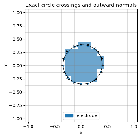

Crossings: 24
First distances from lower edge nodes: [0.06459583 0.03554094 0.05021133 0.11517247 0.02701779 0.05071673
 0.00928327 0.03298221]

Solver-oriented brackets

bracketed_edge_geometry() batches the outside-to-inside edges adjacent to solid nodes. It returns grid-shaped arrays keyed by (axis, side), where side 0 means lower and side 1 means upper; uncut entries are NaN. Fractions are raw and unclamped.

This path assumes one crossing per bracket. It matches the geometry used by Picnic’s current stencil assembly. Its periodic option tests wrapped coordinates. It does not detect an object that lies entirely between fluid nodes.

brackets = bracketed_edge_geometry(grid, [circle])
fractions = np.concatenate([f[np.isfinite(f)] for f in brackets.fractions.values()])
assert np.all((fractions >= 0) & (fractions <= 1))
print("Fluid nodes adjacent to a solid:", brackets.cut.sum())
print("Smallest raw edge fraction:", fractions.min())
plt.hist(fractions, bins=12, edgecolor="black")
plt.xlabel("Raw outside-to-surface fraction")
plt.ylabel("Number of directed cut edges")
plt.show()

Fluid nodes adjacent to a solid: 19
Smallest raw edge fraction: 0.03676662770154948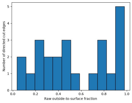

Detect a thin object between fluid nodes

The full cut_edges() inspection visits every edge and can return multiple hits on one edge. Analytic balls, boxes and polygons detect crossings even when both endpoints are outside. General membership functions scan a finite number of samples and may miss narrower features; check cuts.exact and refine samples.

An edge can also be tangent to a surface. intersect_segment() returns such a hit with entering=0; +1 means entering and -1 means leaving.

thin_grid = Grid(
    ndim=2, lower_bound=(0, -0.5), upper_bound=(1, 0.5), num_gridpoints=(2, 3)
)
bead = Circle((0.5, 0), 0.025)
assert not bead.node_mask(thin_grid).any()
thin_cuts = bead.cut_edges(thin_grid)
np.testing.assert_allclose(thin_cuts.fractions, [0.475, 0.525])
print(bead.diagnose(thin_grid))
ax = bead.show(
    bounds=((0, -0.2), (1, 0.2)), resolution=180, display=False, labels=False
)
ax.plot([0, 1], [0, 0], "k.-", label="edge with fluid endpoints")
thin_cuts.show(ax=ax, normals=True, display=False)
ax.legend()
ax.set_title("Two crossings, no solid grid node")
plt.show()

{'overlap_nodes': {}, 'objects_without_solid_nodes': ['geometry'], 'multiple_hit_edges': 1, 'short_distance_hits': 0, 'intersection_search_exact': True, 'scope': 'node and edge samples; does not certify feature resolution'}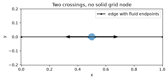

Approximate cell-volume and face-area fractions

cell_fractions() provides a separate geometric quantity: the fraction of each cell (and face) inside the solid. It uses midpoint subcell quadrature, not an exact interface reconstruction. Fluid fractions are one minus these arrays. Increase samples_per_axis to check convergence; features below the sample spacing can be missed.

for samples in (2, 4, 8):
    fractions = circle.cell_fractions(grid, samples_per_axis=samples)
    area = fractions.volume.sum() * np.prod(grid.grid_spacing)
    print(
        f"{samples} samples/axis: area={area:.6f}, exact={np.pi * circle.radius**2:.6f}"
    )
xs, ys = grid.get_grid_points()
plt.pcolormesh(xs, ys, fractions.volume.T, shading="flat", vmin=0, vmax=1, cmap="Blues")
plt.colorbar(label="Solid cell fraction")
plt.gca().set_aspect("equal")
plt.title("Subcell occupancy estimates")
plt.xlabel("x")
plt.ylabel("y")
plt.show()
assert fractions.faces[0].shape == (17, 16)
assert fractions.faces[1].shape == (16, 17)

2 samples/axis: area=0.425781, exact=0.430084
4 samples/axis: area=0.431641, exact=0.430084
8 samples/axis: area=0.429688, exact=0.430084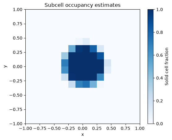

Try moving the circle by a small fraction of one cell and compare the edge fractions. Simgeometry leaves tiny physical distances unchanged. A solver may need to regularize them to control conditioning, which is a discretization decision rather than a geometry tolerance.