xarray
a.to_xarray(dims, ...) gathers an array (like gather/to_numpy) and labels the result as
an xarray.DataArray, for plotting or further analysis with xarray-based tools. It needs
xarray, which is not a dependency of mpiarray; install it separately:
Show code
import numpy as np
import mpiarray as mpa
comm = mpa.default_comm()rank, nranks = comm.Get_rank(), comm.Get_size()
The figures below are generated by this notebook during the docs build with xarray and Matplotlib. Optional plasma-plots cells demonstrate its accessor when installed. Boundary lines reflect the number of MPI ranks actually used: a serial build has no internal rank boundaries.
Show code
from importlib.util import find_spec
plasma_available = find_spec("plasma_plots") is not Noneif plasma_available: pass # registers the xarray accessorelse: print("plasma-plots is optional; the xarray/Matplotlib figures still run.")pip install xarray # or: pip install mpiarray[xarray]xarray is imported on first use only; import mpiarray works without it.
A gathered, labeled array
Section titled “A gathered, labeled array”mpiarray has no notion of what an axis means, so labeled attaches the axis names once,
on the array itself:
import mpiarray as mpa
x = np.linspace(0.0, 1.0, 64)y = np.linspace(0.0, 1.0, 48)rho = mpa.zeros((64, 48), split=0).labeled("x", "y")i0, i1 = rho.layout.index_bounds[0]  # this rank's slab of xxi = np.arange(i0, i1)[:, None] / 64.0 - 0.5yi = np.arange(48)[None, :] / 48.0 - 0.5rho.local[...] = np.exp(-(xi**2 + yi**2) * 20)  # a Gaussian bump
data = rho.to_xarray(x=x, y=y, name="rho")# also: mpa.to_xarray(rho, x=x, y=y, name="rho")
name="rho" above is just a string passed to to_xarray, unrelated to the Python variable
being called rho — naming the variable something else would not change it.
name and general attrs are given at each to_xarray call. If the array has units
attached with set_units, attrs["units"] defaults to their string representation;
an explicit attribute overrides that default.
The coordinate values are optional: rho.to_xarray() alone still gives a DataArray with
dims == ("x", "y") (from labeled), just with no coordinate attached —
Dimensions without coordinates: x, y. Positional selection (isel, or an integer like
component=0 on the .plasma.plot accessor) still works without them; selecting by value
(.sel(), a float like z=0.0 on the accessor, or rank_boundaries, below) needs the real
coordinate to compare against, and raises without it.
labeled returns the array itself (not a copy), so it chains onto any creation call.
a.dims reads back what was set, None if never called; passing dims= explicitly to
to_xarray still works and overrides it for that call. Each coordinate’s values are a
keyword argument named after its axis (x=, y=, …; also any auxiliary coordinate over
the named axes, such as physical X=/Y=/Z= grids over logical eta1/eta2); an axis
named like one of to_xarray’s own parameters (dims, name, attrs, root, coords)
goes through coords= instead, a dict merged with the keyword coordinates.
Elementwise arithmetic, halo updates, copy, astype, redistribute and rebalance keep
the axis names, since which axis is which does not change when the values do; a reshape,
reduction, selection, concatenate or stack drops them, since what the result’s axes mean
is not always obvious — call labeled again on the result if you still want them labeled.
This is collective, like gather: call it on every rank. root= gathers to one rank only
(None, the default: every rank), which matters when handing the result to a plotting
library whose functions only draw on rank 0, such as plasma-plots:
root_data = rho.to_xarray(x=x, y=y, root=0) # every rank calls this# ... then, only on rank 0 (plasma-plots does this for you):# plot_slice(data)Gather before calling into a rank-0-only plotting function, not inside it: those functions
skip their body entirely on the other ranks, so a gather/to_xarray call made only inside
one would hang, waiting for ranks that never call it.
Physical units
Section titled “Physical units”For a worked example, follow the Using physical units guide.
Install mpiarray[units] (or astropy) to enable unit arithmetic. Astropy is imported
only when units are used. set_units labels the existing values without converting them,
returns the same array, and accepts a unit string or an Astropy unit. set_units(None)
clears the unit.
energy = mpa.ones((64, 48)).labeled("x", "y").set_units("eV")volume = mpa.ones((64, 48)).set_units("m3")density = energy / volumeassert str(density.units) == "eV / m3"assert (energy * energy).units == energy.units**2centered = energy - energy.mean()density_data = density.to_xarray(name="energy_density") # attrs["units"] == "eV / m3"Addition, subtraction, comparisons and isclose convert compatible units to the first
operand’s unit, including their numeric scale (for example joules to electronvolts).
Incompatible units raise. Multiplication, division and scalar powers compute the resulting
unit. Bare numbers are dimensionless, so multiplying energy by 2 works, while adding
2 to energy raises; use 2 * astropy.units.eV for a unit-bearing scalar.
sum, mean, min, max, var, std, dot, vdot and norm return host Astropy
Quantities, with variance in squared units. all and any return booleans. copy,
astype, redistribute, rebalance and halo updates preserve units. MPI storage and
local NumPy/CuPy blocks always remain raw arrays; reading or writing .local, gathering,
or calling to_numpy exposes numeric values without a Quantity wrapper.
Indexed assignment converts compatible Quantity or distributed values to the destination
unit and rejects incompatible values before writing. For example, length[:] = 250 * u.cm
writes 2.5 into a metre-valued array. Bare assigned numbers are dimensionless; .local
remains the explicit interface for raw numeric writes. Integer destinations reject
unit-bearing assignments that would lose precision or overflow.
np.isclose and np.allclose accept a physical atol and a dimensionless rtol
(including percent). Bare atol values use the first operand’s unit. Put a distributed
operand first when mixing with a host Quantity in high-level NumPy functions so that
mpiarray handles the call.
allreduce_replicated requires matching units on all ranks: SUM, MIN and MAX keep the
unit; PROD raises it to the number of ranks. Other MPI operations raise for unit-bearing
arrays. A single-rank call is a no-op.
Transcendental functions require dimensionless inputs, rescaling units such as percent
before evaluation. This initial API also requires dimensionless trigonometric inputs;
angle units are not supported. For example, np.exp(energy) and energy + volume raise.
Offset temperature units such as degrees Celsius are unsupported; use kelvin.
Uncategorized elementwise functions, products (prod), axis reductions and index
reductions raise when units are attached. Reshape, selection, concatenation and stacking
currently drop units; reattach them explicitly when their physical meaning is known.
Marking rank boundaries on a plot
Section titled “Marking rank boundaries on a plot”plasma-plots’s plot_slice has an
overlays={"rank_boundaries": ...} option (plasma-plots 0.2.1 and later for passing a
Layout directly, as below; 0.2.0 already took a plain {name: values} dict) that draws
dashed lines where one rank’s block ends and the next begins, styled apart from ordinary
"coordinate_lines" so both can share an axis. Pass the Layout itself, no manual
bookkeeping needed: plasma-plots finds each drawn dimension’s axis by name among the
data’s own dimensions (the sweep dimension, t by default, is skipped) and calls
Layout.boundary_values for it:
import matplotlib.pyplot as plt
# The xarray/Matplotlib path works without an additional plotting package.if rank == 0:    fig, ax = plt.subplots(figsize=(6, 4))    data.plot(ax=ax, x="x", y="y")    for boundary in rho.layout.boundary_values(0, x):        ax.axvline(boundary, color="white", linestyle="--")    ax.set_title("Distributed Gaussian field")    plt.show()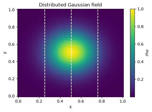
Or with the function form:
if plasma_available and rank == 0:    from plasma_plots.plotting import plot_slice
    plot_slice(data, overlays={"rank_boundaries": rho.layout}).show()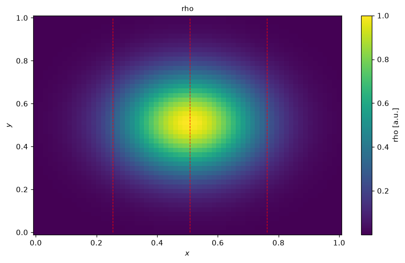
The generated figure above shows the Gaussian bump. Run on four ranks to see three internal boundaries.
For an explicit list of values instead (e.g. lines not tied to any Layout),
Layout.boundary_values(axis, coordinate) turns a layout’s block cuts (Layout.bounds, index
positions) into the coordinate values directly, and overlays takes a plain
{name: values} dict the same way "coordinate_lines" does:
print("cut indices:", rho.layout.bounds[0])print("boundary coordinates:", rho.layout.boundary_values(0, x))cut indices: (0, 16, 32, 48, 64)boundary coordinates: [0.25396825396825395, 0.5079365079365079, 0.7619047619047619]A 3D vector field, sliced and lined out
Section titled “A 3D vector field, sliced and lined out”A “component” axis is labeled like any other:
Show code
import numpy as np
import mpiarray as mpa
nx, ny, nz = 32, 24, 16x = np.linspace(-1.0, 1.0, nx)y = np.linspace(-1.0, 1.0, ny)z = np.linspace(-1.0, 1.0, nz)
E = mpa.zeros((3, nx, ny, nz), split=1).labeled("component", "x", "y", "z")i0, i1 = E.layout.index_bounds[1]  # this rank's slab of x (axis 1: split=1)X, Y, Z = np.meshgrid(x[i0:i1], y, z, indexing="ij")envelope = np.exp(-2.0 * (X**2 + Y**2)) * np.exp(-(Z**2))E.local[0] = -Y * envelope  # ExE.local[1] = X * envelope  # EyE.local[2] = 0.3 * np.sin(np.pi * Z) * envelope  # Ez
data = E.to_xarray(x=x, y=y, z=z, name="E")
data.plasma.plot (registered on every xarray object once plasma-plots is imported) selects
the other axes by naming them: an integer is a position, a float the nearest coordinate
value — component=0 picks Ex, the first of the 3 entries along the "component" axis,
the same way z=0.0 picks the nearest z to 0. A 2-D slice of Ex at z = 0, with the
rank boundaries along x marked:
if rank == 0:    fig, ax = plt.subplots(figsize=(6, 4))    data.isel(component=0).sel(z=0.0, method="nearest").plot(ax=ax, x="x", y="y")    for boundary in E.layout.boundary_values(1, x):        ax.axvline(boundary, color="white", linestyle="--")    ax.set_title("Ex at z = 0")    plt.show()
if plasma_available and rank == 0:    data.plasma.plot.slice(        component=0, z=0.0, title="Ex", overlays={"rank_boundaries": E.layout}    ).show()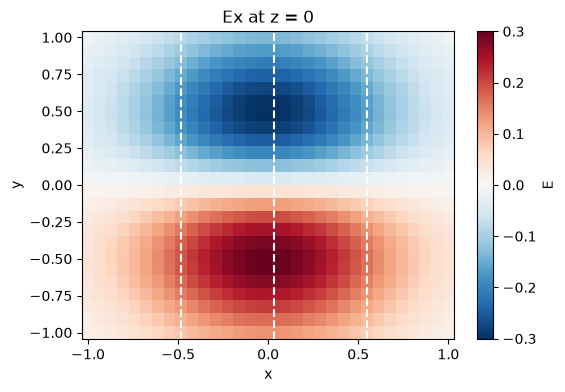
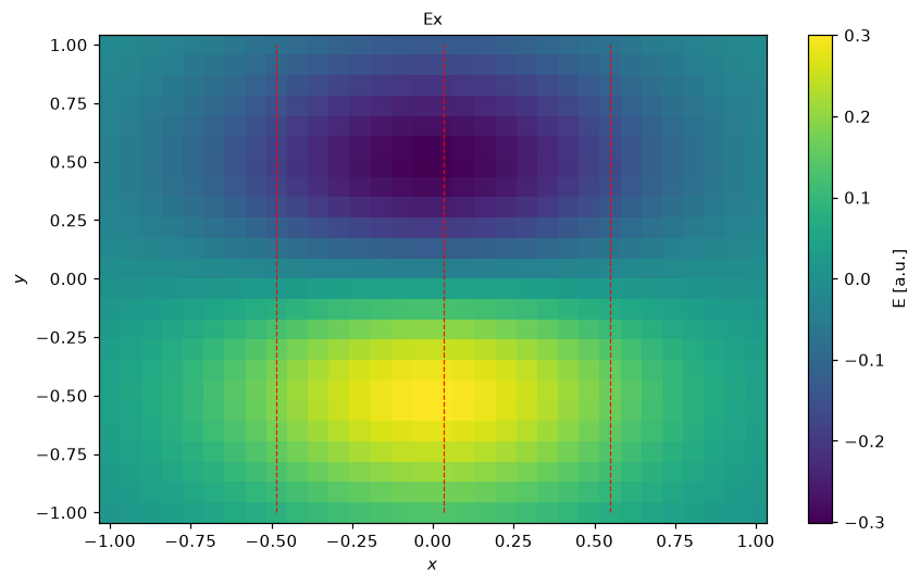
Selecting component=0 does not rename the array, so without title= the plot would just
say "E"; pass it explicitly (here and below) to say which component is shown.
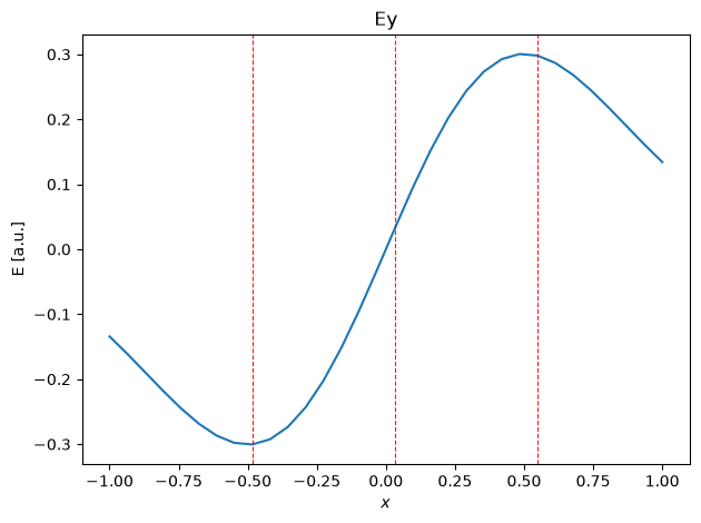
And a 1-D lineout of Ey along x, at y = z = 0, with the same rank boundaries marked
(plot_lineout’s own rank_boundaries= takes a plain list of values; the accessor also
takes a Layout directly here, the same way plot_slice’s does):
if rank == 0:    line = data.isel(component=1).sel(y=0.0, z=0.0, method="nearest")    fig, ax = plt.subplots(figsize=(6, 3))    line.plot(ax=ax, x="x")    for boundary in E.layout.boundary_values(1, x):        ax.axvline(boundary, color="gray", linestyle="--")    ax.set_title("Ey at y = z = 0")    plt.show()
if plasma_available and rank == 0:    data.plasma.plot.lineout(        component=1, y=0.0, z=0.0, title="Ey", rank_boundaries=E.layout    ).show()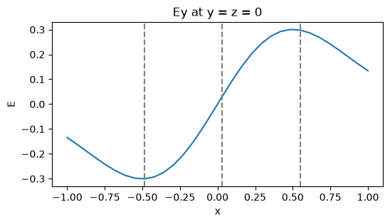
Both need every one of E’s own axes to still be there when plasma-plots sees the data
(Layout.boundary_values is always called with the original array’s axis indices), which
naming axes on the accessor (component=0, z=0.0, …) guarantees: it selects internally,
handing the whole array to plot_slice/plot_lineout. Selecting an axis away yourself
first, e.g. data.isel(component=0), loses that — use plasma_plots.plotting.plot_slice
directly with view=View(isel={"component": 0, ...}) instead in that case, or drop
rank_boundaries.