Domain decomposition
How mpiarray splits an array over the ranks of an MPI job, step by step: the process grid,
the cut points along each axis, the numbering of the ranks and their neighbours, and the
halo cells around every block. The Layouts guide is the
reference for the Layout API; this page explains the decomposition itself, with figures
drawn from mpiarray’s own layouts, and ends with an interactive explorer.
The figures describe runs on 6, 12 or 16 ranks without starting them: a Layout only asks
its communicator for the number of ranks and its own rank, so a small stand-in communicator
is enough to compute what every rank of such a run would own (it cannot communicate). Every
number in the figures comes from Layout.
Show code
import matplotlib.pyplot as pltimport maybempiimport numpy as npfrom matplotlib.colors import to_rgbafrom matplotlib.patches import Rectangle
import mpiarray as mpafrom mpiarray import Layout
comm = mpa.default_comm()rank, nranks = comm.Get_rank(), comm.Get_size()PROC_NULL = maybempi.get_mpi().PROC_NULL  # the "neighbour" beyond a wall

class Ranks:    """A stand-in communicator: the two things `Layout` reads to compute a decomposition.
    Layouts built on it describe what a run on ``size`` ranks would own, without starting    one. They cannot communicate.    """
    def __init__(self, size, rank=0):        self.size, self.rank = size, rank
    def Get_size(self):        return self.size
    def Get_rank(self):        return self.rank

def layouts(size, shape, **options):    """One `Layout` per rank of a run on ``size`` ranks, each knowing its own neighbours."""    return [Layout(shape, comm=Ranks(size, r), **options) for r in range(size)]

# one colour per rank, the same as in the explorer at the end of the pagePALETTE = [    "#1f77b4",    "#ff7f0e",    "#2ca02c",    "#d62728",    "#9467bd",    "#8c564b",    "#e377c2",    "#7f7f7f",    "#bcbd22",    "#17becf",    "#aec7e8",    "#ffbb78",    "#98df8a",    "#ff9896",    "#c5b0d5",    "#c49c94",    "#f7b6d2",    "#c7c7c7",    "#dbdb8d",    "#9edae5",]ACCENT = "#2a78d6"WALL = {    "facecolor": "#ededed",    "hatch": "///",    "edgecolor": "#9a9a9a",    "linewidth": 0.5,}

def rank_color(r):    return PALETTE[r % len(PALETTE)]

def owner_map(layout):    """The rank that owns every cell of a 2-D layout, as an array of the global shape."""    n0, n1 = layout.shape    i, j = np.meshgrid(np.arange(n0), np.arange(n1), indexing="ij")    return layout.owners(np.stack([i, j], axis=-1))

def caption(ax, text):    ax.text(0.5, -0.04, text, transform=ax.transAxes, ha="center", va="top", fontsize=9)

def draw_blocks(    ax, layout, *, coords=False, cells=True, caption_text=None, fontsize=11):    """Colour the cells of a 2-D array by the rank that owns them and draw the cuts."""    n0, n1 = layout.shape    if layout.replicated:        image = np.broadcast_to(to_rgba("#d8d8d8", 0.8), (n0, n1, 4))    else:        colors = np.array([to_rgba(rank_color(r), 0.65) for r in range(layout.size)])        image = colors[owner_map(layout)]    ax.imshow(image, extent=(0, n1, n0, 0), interpolation="nearest")    if cells:        ax.set_xticks(np.arange(n1 + 1), minor=True)        ax.set_yticks(np.arange(n0 + 1), minor=True)        ax.grid(which="minor", color="white", linewidth=0.6)    ax.grid(which="major", visible=False)    ax.hlines(layout.bounds[0], 0, n1, color="black", linewidth=1.8)... (156 lines skipped) ...    )    ax.add_patch(block)    ax.add_patch(        Rectangle((0, 0), m1, m0, fill=False, edgecolor="black", linestyle="--")    )    ax.set_xticks(sorted({0, h1, m1 - h1, m1}))    ax.set_yticks(sorted({0, h0, m0 - h0, m0}))    ax.tick_params(which="both", length=0)    ax.xaxis.tick_top()    ax.xaxis.set_label_position("top")    ax.set(xlabel="storage index, axis 1", ylabel="storage index, axis 0")    ax.text(        m1 / 2,        m0 / 2,        f"local\nrank {layout.rank}",        ha="center",        va="center",        fontsize=fontsize,    )

def draw_neighbours(ax, layout, margin=2.5):    """Arrows from this rank's block to its neighbours along each axis, leaving the array where they wrap around."""    (a0, a1), (b0, b1) = layout.index_bounds    n0, n1 = layout.shape    ax.add_patch(        Rectangle((b0, a0), b1 - b0, a1 - a0, fill=False, edgecolor=ACCENT, linewidth=3)    )    arrow = {        "arrowstyle": "-|>",        "color": "black",        "linewidth": 1.5,        "shrinkA": 0,        "shrinkB": 0,    }    out0, out1 = (        margin - 0.7,        margin - 0.7,    )  # how far the wrap-around arrows leave the array    tags = {}    for axis, pair in enumerate(layout.neighbours):        for step, neighbour in zip((-1, 1), pair, strict=True):            if neighbour == PROC_NULL:                x, y = (b0 + b1) / 2, (a0 + a1) / 2                if axis == 0:                    y = -out0 if step < 0 else n0 + out0                else:                    x = -out1 if step < 0 else n1 + out1                rotation = 0 if axis == 0 else 90                ax.text(                    x,                    y,                    "PROC_NULL",                    ha="center",                    va="center",                    fontsize=8,                    color="gray",                    rotation=rotation,                )                continue            (c0, c1), (d0, d1) = layout.index_bounds_of(neighbour)            if axis == 0:                x = (b0 + b1) / 2                start, end = (                    (x, a0 if step < 0 else a1),                    ((d0 + d1) / 2, c1 if step < 0 else c0),                )                adjacent = (c1 == a0) if step < 0 else (c0 == a1)                exit_point = (x, -out0 if step < 0 else n0 + out0)                entry = (end[0], n0 + out0 if step < 0 else -out0)            else:                y = (a0 + a1) / 2                start, end = (                    (b0 if step < 0 else b1, y),                    (d1 if step < 0 else d0, (c0 + c1) / 2),                )                adjacent = (d1 == b0) if step < 0 else (d0 == b1)                exit_point = (-out1 if step < 0 else n1 + out1, y)                entry = (n1 + out1 if step < 0 else -out1, end[1])            if adjacent:                ax.annotate("", xy=end, xytext=start, arrowprops=arrow)            else:  # wrap-around: out of the array on this side, in again on the other                ax.annotate("", xy=exit_point, xytext=start, arrowprops=arrow)                ax.annotate("", xy=end, xytext=entry, arrowprops=arrow)            if neighbour != layout.rank:                tags.setdefault(neighbour, []).append(                    f"axis {axis} {'−' if step < 0 else '+'}"                )    for neighbour, names in tags.items():        (c0, c1), (d0, d1) = layout.index_bounds_of(neighbour)        ax.text(            (d0 + d1) / 2,            (c0 + c1) / 2 + 2.2,            ", ".join(names),            ha="center",            va="center",            fontsize=8,            fontweight="bold",        )    ax.set(xlim=(-margin, n1 + margin), ylim=(n0 + margin, -margin))
One array, one block per rank
Section titled “One array, one block per rank”A distributed array is one global array of which every rank stores one block: a box of
global indices, layout.index_bounds, with nothing in common with the other ranks’ boxes.
The blocks tile the array, so every cell has exactly one owner, layout.owner(index). Here
a array is split over 6 ranks along both axes:
layout = layouts(6, (12, 9), split=(0, 1))[0]  # what rank 0 of a run on 6 ranks sees
fig, (left, right) = plt.subplots(1, 2, figsize=(9, 4.4))draw_blocks(left, layout, caption_text="the global array, coloured by owner")draw_exploded(right, layout)caption(right, "the block each rank stores (its local_shape)")plt.show()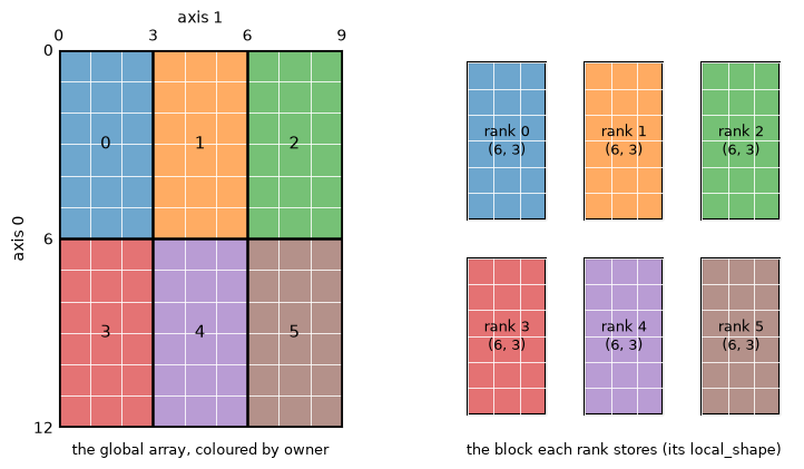
The decomposition is decided in two steps, each explained below:
- The process grid: how many ranks go along each axis ( here), so that the ranks form a grid of the same number of dimensions as the array.
- The cut points: along every axis, where one rank’s index range ends and the next
begins (
layout.bounds, here(0, 6, 12)and(0, 3, 6, 9)). A rank’s block is the product of one piece per axis.
Then every rank is given a position on the grid, from which its neighbours follow, and stores its block with a frame of halo cells.
The process grid
Section titled “The process grid”split names the axes to cut; the default is axis 0 only. The ranks are shared among the
split axes as evenly as divisibility allows, by mpa.process_grid, which only looks at the
number of ranks and the split axes, not at the shape. On two split axes:
fig, axes = plt.subplots(4, 4, figsize=(9, 9.6))for size, ax in zip(range(1, 17), axes.flat, strict=True): grid = layouts(size, (24, 24), split=(0, 1))[0] draw_blocks(ax, grid, cells=False, fontsize=8) g0, g1 = grid.process_grid ax.set(xlabel=None, ylabel=None, xticks=[], yticks=[]) caption(ax, f"{size} ranks: {g0} × {g1}")fig.tight_layout()plt.show()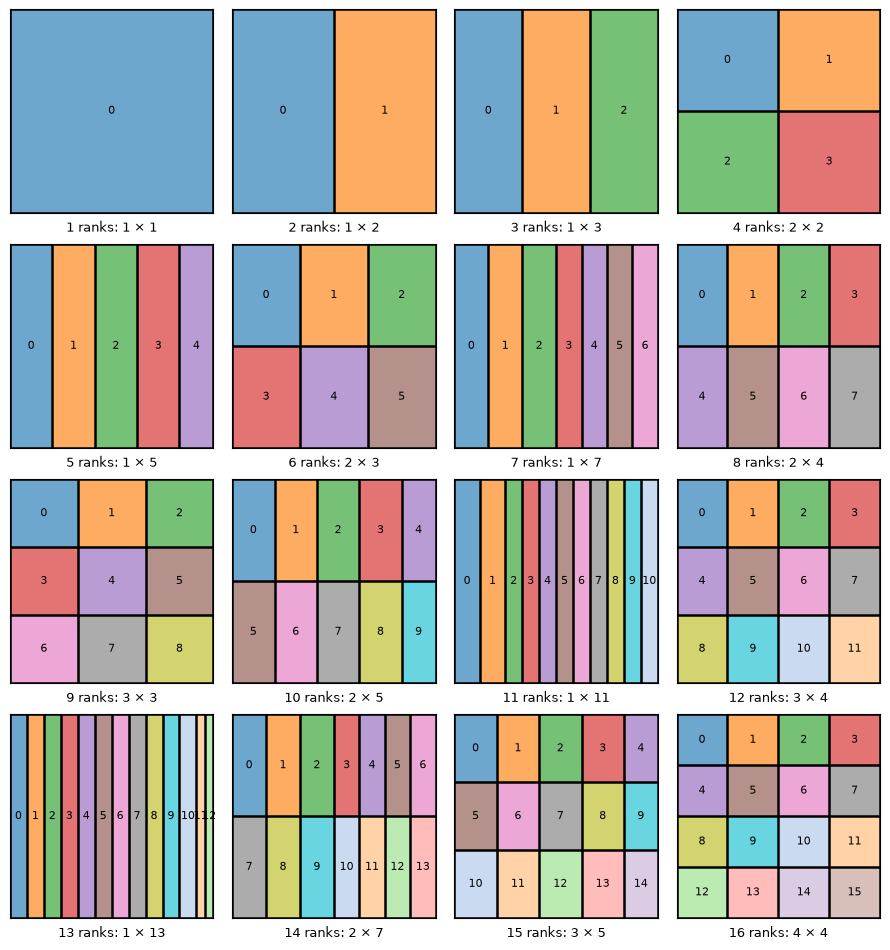
The split axes are filled in order. With split axes left to fill and ranks left to place, the next axis gets the largest divisor of that is not above , and the last axis takes what remains, so the product is always the number of ranks. ranks give , give ; a prime number of ranks cannot be shared, so or ranks all go to the last split axis. Rank counts with small factors () give balanced grids.
Which axes are split decides the shape of the blocks. On 6 ranks, the same
array with split=0, split=1, split=(0, 1), and split=None, where no axis is split
and every rank holds the whole array (a replicated layout):
fig, axes = plt.subplots(1, 4, figsize=(11, 3.8))for ax, split in zip(axes, (0, 1, (0, 1), None), strict=True): grid = layouts(6, (12, 9), split=split)[0] draw_blocks(ax, grid, fontsize=9) caption(ax, f"split={split}: process grid {grid.process_grid}") if ax is not axes[0]: ax.set(ylabel=None, yticks=[])plt.show()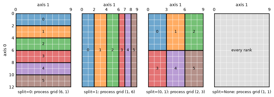
Choosing the grid yourself
Section titled “Choosing the grid yourself”Because the automatic grid ignores the shape, an elongated array can get blocks that are
long and thin, with large faces between them. Every face is a surface through which halo
cells are exchanged at each update_halos(): the figure counts, for a array
on 12 ranks with one halo layer, the cells every grid receives per update, summed over the
ranks. The automatic grid is ; process_grid= chooses any other factorisation
(its product must be the number of ranks, and its axes with more than one rank become the
split axes):
def halo_cells_received(size, shape, **options):    """Cells that update_halos() fills on all ranks together: halo cells with a neighbour."""    return sum(        int(np.count_nonzero((sources != lay.rank) & (sources >= 0)))        for lay in layouts(size, shape, **options)        for sources in [storage_sources(lay)]    )

fig, axes = plt.subplots(1, 6, figsize=(12, 4.2))for ax, grid in zip(    axes, [(12, 1), (6, 2), (4, 3), (3, 4), (2, 6), (1, 12)], strict=True):    lay = layouts(12, (48, 24), process_grid=grid, halo=1)[0]    draw_blocks(ax, lay, cells=False, fontsize=8)    received = halo_cells_received(12, (48, 24), process_grid=grid, halo=1)    automatic = " (automatic)" if grid == (4, 3) else ""    caption(ax, f"{grid[0]} × {grid[1]}{automatic}\n{received} halo cells")    ax.set(xlabel=None, ylabel=None)fig.tight_layout()plt.show()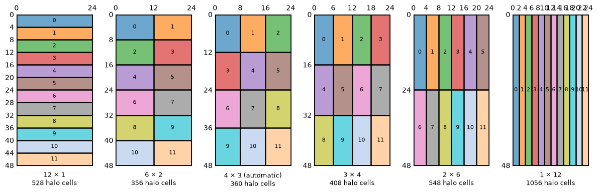
Blocks close to square exchange the least: and both give blocks of
or cells, while the strips of and
exchange up to three times as much. Give the most ranks to the longest axis, and leave
unsplit the axes that are short or that an algorithm needs whole on every rank (a component
axis of a vector field, an axis you transform with an FFT). halo=(2, 2, 0) likewise gives
no halo cells along an axis that is not split.
Cutting each axis
Section titled “Cutting each axis”Along a split axis of length shared by ranks, rank (counted along that axis) gets
the half-open index range mpa.chunk_bounds(L, n, i): every rank gets elements, and the first ranks one more, so the lengths differ by at most
one. An axis of 10 elements on 1 to 6 ranks:
length = 10fig, axes = plt.subplots(6, 1, figsize=(8, 4.4), sharex=True)for n, ax in zip(range(1, 7), axes, strict=True): for i in range(n): start, end = mpa.chunk_bounds(length, n, i) ax.add_patch( Rectangle((start, 0), end - start, 1, facecolor=rank_color(i), alpha=0.65) ) ax.add_patch( Rectangle((start, 0), end - start, 1, fill=False, edgecolor="black") ) ax.text((start + end) / 2, 0.5, str(end - start), ha="center", va="center") ax.set(xlim=(0, length), ylim=(0, 1), yticks=[]) ax.set_ylabel(f"{n} ranks", rotation=0, ha="right", va="center") ax.grid(visible=False)axes[-1].set(xticks=range(length + 1), xlabel="global index")plt.show()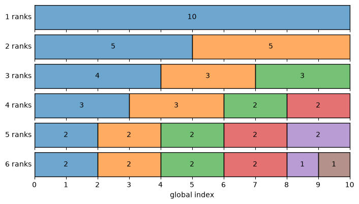
The numbers in the blocks are their lengths: with 4 ranks, . Each axis
is cut on its own, and layout.bounds collects the cut points of all axes: along each one,
the global index where every block starts, and the length. A block is the product of one
piece per axis, so the cuts of a array on ranks are two short
tuples:
lay = layouts(4, (10, 7), split=(0, 1))[0]print("process grid:", lay.process_grid)print("bounds:      ", lay.bounds)for r in range(4):    print(        f"rank {r} owns rows {lay.index_bounds_of(r)[0]} and columns {lay.index_bounds_of(r)[1]}"    )
fig, ax = plt.subplots(figsize=(3.6, 4.4))draw_blocks(ax, lay)caption(ax, "ticks: where the blocks start, and the length")plt.show()
process grid: (2, 2)bounds: ((0, 5, 10), (0, 4, 7))rank 0 owns rows (0, 5) and columns (0, 4)rank 1 owns rows (0, 5) and columns (4, 7)rank 2 owns rows (5, 10) and columns (0, 4)rank 3 owns rows (5, 10) and columns (4, 7)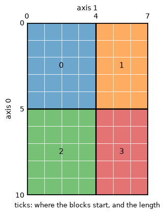
When the ranks do not fit
Section titled “When the ranks do not fit”A split axis needs at least as many elements as ranks along it, and every halo must fit in
the smallest block of its axis (a halo is filled from the neighbouring block only).
Otherwise Layout, and every creation function, raises a ValueError on every rank rather
than leaving a rank without cells:
try: Layout( (3, 40), comm=Ranks(16), split=0 ) # only axis 0 may be cut: 3 elements, 16 ranksexcept ValueError as error: print("ValueError:", error)try: Layout(10, comm=Ranks(4), halo=3) # blocks of 3, 3, 2 and 2 elementsexcept ValueError as error: print("ValueError:", error)ValueError: axis 0 has 3 elements but is split over 16 ranks; use fewer ranks, split=None, another split axis, or a process_gridValueError: halo 3 along axis 0 is wider than the smallest block (2 elements); use a smaller halo or fewer ranksWhen the automatic grid is the problem, Layout first looks for another grid: if
process_grid’s choice gives an axis more ranks than elements, the layout takes, of all the
grids that fit, the one with the smallest halo surface. A array on 16 ranks
with split=(0, 1) would get , which does not fit; of the grids that do,
has the smallest faces and is chosen over :
fig, axes = plt.subplots(2, 1, figsize=(11, 3.6))for ax, grid in zip(axes, [None, (2, 8)], strict=True): options = {"split": (0, 1)} if grid is None else {"process_grid": grid} lay = layouts(16, (3, 40), halo=1, **options)[0] draw_blocks(ax, lay, fontsize=8) received = halo_cells_received(16, (3, 40), halo=1, **options) chosen = ( "chosen: the smallest halo surface" if grid is None else "process_grid=(2, 8)" ) caption( ax, f"{lay.process_grid[0]} × {lay.process_grid[1]}, {received} halo cells ({chosen})", ) ax.set(xlabel=None, ylabel=None)fig.tight_layout()plt.show()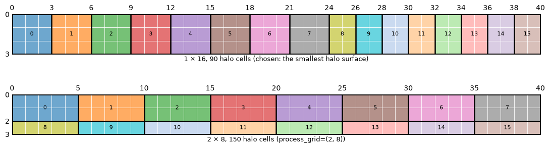
Ranks on the grid
Section titled “Ranks on the grid”Every rank has a position on the process grid, layout.process_coord, and the ranks are
placed in row-major order: the last axis varies fastest, like the elements of a C-ordered
array. On a grid, rank sits at coordinates , and the rank at is ; layout.coord_of and layout.rank_of
convert between the two.
lay = layouts(12, (24, 32), split=(0, 1))[0]print("process grid:", lay.process_grid)print("rank 5 sits at", lay.coord_of(5), "and", lay.rank_of((1, 1)), "sits at (1, 1)")print("cell (7, 4) belongs to rank", lay.owner((7, 4)))
fig, ax = plt.subplots(figsize=(6, 5))draw_blocks(ax, lay, coords=True, cells=False)caption(ax, "rank and process coordinates of every block")plt.show()
process grid: (3, 4)rank 5 sits at (1, 1) and 5 sits at (1, 1)cell (7, 4) belongs to rank 0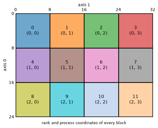
The rank is the one in the layout’s communicator, MPI.COMM_WORLD by default, so the MPI
launcher decides which process gets which block. With Layout(..., reorder=True) the layout
asks MPI for a Cartesian communicator instead (MPI_Cart_create with reordering), which may
renumber the ranks so that neighbouring blocks land on nearby cores; the layout’s comm,
rank and neighbours then refer to that communicator.
Neighbours, periodicity and walls
Section titled “Neighbours, periodicity and walls”layout.neighbours gives, for every axis, the pair of ranks whose blocks come just before
and just after this rank’s along that axis. Inside the grid they are the adjacent blocks;
at the ends of an axis, periodic decides: along a periodic axis the neighbour is the
block at the other end of the array, and along a non-periodic one there is a wall, marked
by MPI.PROC_NULL. MPI calls with PROC_NULL do nothing, so halo code needs no special
case for walls.
fig, axes = plt.subplots(1, 3, figsize=(12, 4.6))cases = [(5, (True, True)), (0, (True, True)), (0, (False, False))]for ax, (r, periodic) in zip(axes, cases, strict=True): lay = layouts(12, (24, 32), split=(0, 1), periodic=periodic)[r] draw_blocks(ax, lay, cells=False, fontsize=9) draw_neighbours(ax, lay) caption(ax, f"rank {r}, periodic={periodic}\nneighbours {lay.neighbours}")fig.tight_layout()plt.show()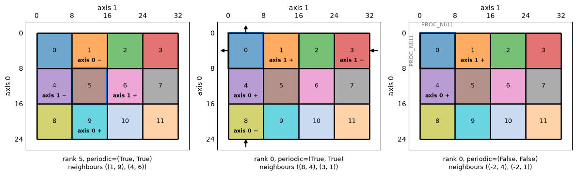
Rank 5 sits inside the grid, so its neighbours are the same whatever the periodicity. Rank 0
is in a corner: with periodic axes its lower neighbours are the blocks at the far ends (the
arrows leave the array and come back on the other side), without them they are walls
(PROC_NULL, a negative number in the tuples above: under Open MPI, under MPICH).
With
only two ranks along an axis the two neighbours are the same rank, and with one rank along a
periodic axis a rank is its own neighbour.
Only the neighbours along the axes are listed. The diagonal neighbours, which fill the
corner halo cells, are reached either through two exchanges, one per axis, or directly with
update_halos(wait=False).
Halo cells: what each rank stores
Section titled “Halo cells: what each rank stores”Each rank stores its block with halo[axis] extra cells on both sides of every axis, in one
NumPy or CuPy array of layout.storage_shape: a.local_with_halos is the whole storage,
a.local the block inside it (layout.interior is the slice between the two). The halo
cells are copies of the neighbours’ boundary cells, filled by update_halos(), and
accumulate_halos() adds them into the neighbours’ cells instead.
The figure shows a array on ranks with two halo layers, periodic along axis 0 and with walls along axis 1. On the left, the halo cells of one rank are marked in the global array; on the right, that rank’s storage, with every halo cell coloured by the rank it is filled from:
fig, axes = plt.subplots(2, 2, figsize=(9, 9), gridspec_kw={"width_ratios": [1.15, 1]})for (left, right), r in zip(axes, (4, 0), strict=True): lay = layouts(9, (12, 12), split=(0, 1), halo=2, periodic=(True, False))[r] draw_blocks(left, lay, fontsize=9) draw_halo(left, lay) caption(left, f"the halo cells of rank {r} in the global array") draw_storage(right, lay) caption( right, f"the storage of rank {r}: {lay.storage_shape} for a {lay.local_shape} block", )fig.tight_layout()plt.show()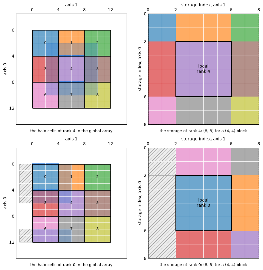
Rank 4, in the middle, is filled from all eight neighbours, the corners from the diagonal
ones. Rank 0 is in a corner: along the periodic axis 0 its upper halo rows wrap around and
come from rank 6 at the bottom of the array, while along axis 1 its left halo columns lie
beyond a wall (hatched): no neighbour fills them, so update_halos() leaves them as they
are, unless a boundary= condition is given, and accumulate_halos() drops what is written
into them. The halo exchange guide covers both
operations and the boundary conditions.
This is also why a halo must not be wider than the smallest block along its axis: the halo cells are filled from the neighbouring block only, not from the one behind it.
Uneven blocks
Section titled “Uneven blocks”The near-even cut is the default, not a requirement. Three ways to cut differently; the ranks are still placed row-major on the grid, and neighbours and halo cells work the same:
bounds=gives the cut points per axis directly (Nonefor an axis that is not split); the process grid follows from them.layout.aligned(shape)makes a layout for another shape whose blocks start where this one’s do, for arrays that belong together but differ in length: the values at the cells and the nodes of a grid, so that cell and node are on the same rank.Layout.weighted(shape, weights)cuts each axis so that every block gets about the same share of a cost, for load balancing.
uneven = Layout((10, 6), comm=Ranks(3), bounds=[(0, 2, 5, 10), None])cells = Layout(16, comm=Ranks(4))nodes = cells.aligned(17)print("uneven bounds:", uneven.bounds)print("cells:", cells.bounds, " nodes:", nodes.bounds)
fig, ax = plt.subplots(figsize=(3.2, 4.4))draw_blocks(ax, uneven, fontsize=9)caption(ax, "bounds=[(0, 2, 5, 10), None] on 3 ranks")plt.show()
fig, ax = plt.subplots(figsize=(9, 2.2))for r in range(4):    ((a0, a1),) = cells.index_bounds_of(r)    ax.add_patch(Rectangle((a0, 0), a1 - a0, 1, facecolor=rank_color(r), alpha=0.65))    ax.add_patch(Rectangle((a0, 0), a1 - a0, 1, fill=False, edgecolor="black"))    ((b0, b1),) = nodes.index_bounds_of(r)    ax.scatter(        np.arange(b0, b1),        np.full(b1 - b0, 1.5),        s=70,        color=rank_color(r),        edgecolor="black",        zorder=3,    )ax.set(xlim=(-0.5, 17.5), ylim=(-0.3, 2.0), yticks=[0.5, 1.5], xticks=range(0, 17, 2))ax.set_yticklabels(["cells: Layout(16)", "nodes: .aligned(17)"])ax.set_xlabel("global index")ax.grid(visible=False)plt.show()
uneven bounds: ((0, 2, 5, 10), (0, 6))cells: ((0, 4, 8, 12, 16),) nodes: ((0, 4, 8, 12, 17),)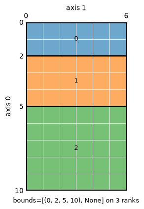
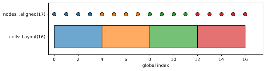
Cell and node are on the same rank, and the last block takes the extra node.
Layout.weighted sums the weights over the other axes to get one cost profile per split
axis and places the cuts where the cumulative cost crosses equal shares (a block keeps at
least one element, and at least its halo width). When the first rows of a
array cost three times as much as the rest, for example because more particles live there,
the near-even cut leaves rank 0 with nearly half the total cost, and the weighted one evens it out:
n = 24cost = np.ones((n, n))cost[:8] = 3.0  # the first 8 rows cost three times as much per celleven = layouts(4, (n, n))[0]balanced = Layout.weighted((n, n), cost, comm=Ranks(4))print("near-even rows:", even.bounds[0], " weighted rows:", balanced.bounds[0])
fig, axes = plt.subplots(    1, 3, figsize=(11, 3.9), gridspec_kw={"width_ratios": [1, 1, 1.1]})for ax, lay, title in zip(    axes[:2], (even, balanced), ("near-even", "Layout.weighted"), strict=True):    ax.imshow(cost, cmap="Greys", vmin=0, vmax=4, extent=(0, n, n, 0))    for c in lay.bounds[0][1:-1]:        ax.axhline(c, color=ACCENT, linewidth=2.5)    for r in range(4):        (a0, a1), _ = lay.index_bounds_of(r)        ax.text(            n / 2,            (a0 + a1) / 2,            f"rank {r}",            ha="center",            va="center",            color="white",            fontsize=9,        )    ax.set(xticks=[], yticks=lay.bounds[0], ylabel="axis 0")    ax.grid(visible=False)    caption(ax, f"{title}: cuts at {lay.bounds[0]}")totals = {    name: [cost[slice(*lay.index_bounds_of(r)[0])].sum() for r in range(4)]    for name, lay in (("near-even", even), ("weighted", balanced))}x = np.arange(4)axes[2].bar(x - 0.2, totals["near-even"], 0.4, label="near-even", color="#b0b0b0")axes[2].bar(x + 0.2, totals["weighted"], 0.4, label="weighted", color=ACCENT)axes[2].set(xticks=x, xlabel="rank", ylabel="total cost of the block")axes[2].legend()fig.tight_layout()plt.show()
near-even rows: (0, 6, 12, 18, 24) weighted rows: (0, 3, 7, 14, 24)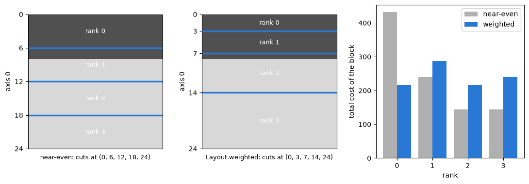
a.rebalance(weights) redistributes an existing array to such a layout, and
a.redistribute(layout) to any other layout of the same shape, in one Alltoallv; see
Changing the layout. Arrays combine
elementwise only when their layouts are equal, cut points included.
The decomposition of this run
Section titled “The decomposition of this run”Everything above is computed by Layout from the number of ranks, so the real thing looks
the same. This notebook runs on several ranks when the docs are built; the cell below asks
each rank for its block and neighbours (allgather is collective, so every rank calls it)
and draws the layout of this run:
a = mpa.zeros((12, 9), split=(0, 1), halo=1, periodic=(True, False))layout = a.layoutrows = comm.allgather(    (layout.rank, layout.process_coord, layout.index_bounds, layout.neighbours))

def name(neighbour):    return "wall" if neighbour == PROC_NULL else str(neighbour)

if rank == 0:    print(        f"{nranks} rank(s), process grid {layout.process_grid}, bounds {layout.bounds}"    )    for r, coord, bounds, neighbours in sorted(rows):        pairs = ", ".join(f"({name(lo)}, {name(hi)})" for lo, hi in neighbours)        print(f"rank {r} at {coord} owns {bounds}; neighbours {pairs}")    fig, ax = plt.subplots(figsize=(4, 4.8))    draw_blocks(ax, layout, coords=True)    caption(ax, f"this run: {nranks} rank(s), {a.layout.local_shape} cells on rank 0")    plt.show()
4 rank(s), process grid (2, 2), bounds ((0, 6, 12), (0, 5, 9))rank 0 at (0, 0) owns ((0, 6), (0, 5)); neighbours (2, 2), (wall, 1)rank 1 at (0, 1) owns ((0, 6), (5, 9)); neighbours (3, 3), (0, wall)rank 2 at (1, 0) owns ((6, 12), (0, 5)); neighbours (0, 0), (wall, 3)rank 3 at (1, 1) owns ((6, 12), (5, 9)); neighbours (1, 1), (2, wall)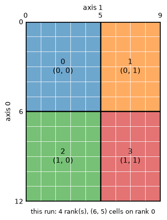
Explore
Section titled “Explore”The explorer below applies the same rules in the browser: choose the number of ranks, the
shape, the split axes, the halo width, the periodicity and, instead of the automatic
process grid, any other factorisation. Hover a block to see that rank’s process coordinates,
index bounds, storage and neighbours (click to keep it); the dashed cells are its halo
cells, and the arrows point to the neighbours that fill them. Settings that mpiarray rejects
show the ValueError it would raise.
the global array, coloured by the rank that owns each cell
one rank's storage
Hover a block to see that rank's view; click to keep it. Dashed: the halo cells of the selected rank; hatched: halo cells outside a wall, which no neighbour fills.
Summary
Section titled “Summary”| Step | Decided by | Read from the layout |
|---|---|---|
| ranks per axis | split and the number of ranks (mpa.process_grid), or process_grid=; a fitting grid if that one does not fit | process_grid |
| cut points per axis | mpa.chunk_bounds, or bounds=, aligned, Layout.weighted | bounds, index_bounds, owner, owners |
| position of each rank | row-major over the grid, or MPI with reorder=True | rank, process_coord, coord_of, rank_of |
| neighbours | adjacent blocks; periodic at the ends, else PROC_NULL | neighbours |
| storage | the block plus halo cells on both sides of every axis | local_shape, storage_shape, interior |
Next: Halo exchange moves data through the halo cells, and the heat equation puts the decomposition to work.