Tutorial 5 - 3D plotting

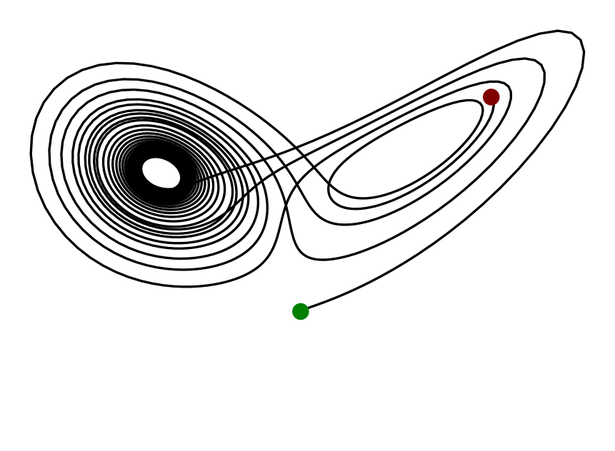
This tutorial draws a Lorenz System, it reproduces a tutorial from Tikz-Python.

%load_ext autoreload
%autoreload 2

from tikzpics import TikzFigure

# source: https://github.com/ltrujello/Tikz-Python/blob/main/examples/lorenz/lorenz.py
import numpy as np
from scipy.integrate import odeint

# lorenz parameters
rho = 28.0
sigma = 10.0
beta = 8.0 / 3.0


# Next state according to the ODEs
def next(*state):
    x, y, z = state[0][0], state[0][1], state[0][2]
    return sigma * (y - x), x * (rho - z) - y, x * y - beta * z


# Set initial conditions and time steps
initial = [1.0, 1.0, 1.0]
t = np.arange(0.0, 20.0, 0.01)

# Solve for the next positions, scale them
states = odeint(func=next, y0=initial, t=t)
states = states * 0.25

xvec = states[:, 0]
yvec = states[:, 1]
zvec = states[:, 2]

# Plot the lorenz system
fig = TikzFigure(ndim=3)
options = ["color=black", "thick"]

fig.plot3d(xvec, yvec, zvec, options=options, layer=0)
fig.add_node(
    x=xvec[0],
    y=yvec[0],
    z=zvec[0],
    fill="green!50!black",
    inner_sep="2.0pt",
    options="circle",
)
fig.add_node(
    x=xvec[-1],
    y=yvec[-1],
    z=zvec[-1],
    fill="red!50!black",
    inner_sep="2.0pt",
    options="circle",
)

fig.show(width=500)