This is the full developer documentation for plasma-plots # Getting started > Install plasma-plots and make your first plot. ## Installation [Section titled “Installation”](#installation) Python **3.10 or newer** is required; CI tests Python 3.10 to 3.14. The base install plots in-memory xarray data. Install extras for file formats and optional renderers: ```bash pip install plasma-plots pip install "plasma-plots[netcdf]" pip install "plasma-plots[netcdf,plotly]" ``` | Extra | Enables | Dependencies | | ----------- | ---------------------------------------------------------------- | ---------------------------------------------------- | | `netcdf` | Read netCDF3/netCDF4 files through xarray and the CLI | `netCDF4` | | `plotly` | Interactive browser plots and static Plotly exports | `plotly`, `kaleido` | | `tikz` | TikZ/pgfplots versions of the plots for LaTeX (`backend="tikz"`) | `maxplotlibx` (and `pdflatex` to compile) | | `pyvista` | 3-D scenes and rendering | `pyvista`, `imageio` | | `profiling` | Timing summaries and profiling plots | `scope-profiler[pproc]` | | `desc` | Evaluate DESC equilibria | `desc-opt` | | `gallery` | Export Struphy example-gallery figures and profiling | `plotly`, `kaleido`, `scope-profiler[pproc]>=0.6.1` | | `dev` | Tests, linting and documentation tooling | `pytest`, `ruff`, `h5py`, `griffe`, `struphy>=3.4.0` | Struphy is installed by the `dev` extra; otherwise install it separately as described below. GVEC and Zarr are separate installations. Install `gvec` for GVEC evaluation or `zarr` to open Zarr stores. MP4 export requires system `ffmpeg`; Matplotlib windows require a working GUI/display, and static Plotly exports through Kaleido require a compatible Chrome installation. ## Struphy compatibility [Section titled “Struphy compatibility”](#struphy-compatibility) Struphy integration requires **Struphy 3.4.0 or newer** from PyPI: ```bash pip install "struphy>=3.4.0" ``` Struphy is optional when working with ordinary xarray data. ## Loading plasma-plots [Section titled “Loading plasma-plots”](#loading-plasma-plots) Creating a Struphy `Output` loads plasma-plots, so there is nothing to import: ```python from struphy.post_processing.output import Output out = Output("path/to/run") out.plot.energies() # whole-run plots and diagnostics field = out.evaluate("em_fields/phi") field.plasma.plot.slice(x="eta1", y="eta2", t=-1) # .plasma on every product ``` Loading it registers the accessors: * `.plasma` on every `xarray.DataArray` and `xarray.Dataset`, including the products of Struphy’s `Output` and every array derived from them * `out.plot` and `out.analysis` on Struphy’s `Output` object Other xarray data: `import plasma_plots` For xarray data that doesn’t come from an `Output` (your own arrays, or files opened with xarray), import the package first: ```python import plasma_plots # noqa: F401 (registers DataArray.plasma) ``` Without it, `.plasma` does not exist and you get `AttributeError: 'DataArray' object has no attribute 'plasma'`. The import alone does the work, so linters may flag it as unused. ## Data from other codes [Section titled “Data from other codes”](#data-from-other-codes) plasma-plots reads labeled `xarray` objects, not a file format, so the output of any code works once it is an array with named dimensions and coordinates. The names follow Struphy’s: | Name | What | | ---------------------- | ------------------------------------------------------------------------------------------------------------ | | `t` | time | | `eta1`, `eta2`, `eta3` | logical coordinates in \[0, 1] | | `X`, `Y`, `Z` | mapped (physical) coordinates, as coordinates over the logical dimensions; all three for `coords="physical"` | | `component` | the components of a vector field | | `marker` | the markers of particle Datasets | [GVEC](https://gvec.readthedocs.io)’s evaluations (dimensions `rad`, `pol`, `tor`) are read in these conventions by themselves, with the flux coordinates `rho`, `theta`, `zeta` as the logical dimensions; see [GVEC equilibria](/plasma-plots/guides/gvec/). Other dimension names work wherever you name the dimensions yourself (`x="z"`, `y="t"`); only the physical views and the mapped-domain analysis need `X`/`Y`/`Z`. The `label` and `units` attributes of the array and the `long_name` and `units` of its coordinates become the axis labels: ```python import numpy as np import xarray as xr import plasma_plots # noqa: F401 t, eta1, eta2 = ( np.linspace(0, 10, 41), np.linspace(0, 1, 32), np.linspace(0, 1, 24, endpoint=False), ) r, theta = 0.2 + 0.8 * eta1[:, None], 2 * np.pi * eta2[None, :] phi = xr.DataArray( np.exp(-0.1 * t)[:, None, None] * np.cos(2 * np.pi * eta1)[None, :, None] * np.cos(theta)[None], dims=("t", "eta1", "eta2"), coords={ "t": t, "eta1": eta1, "eta2": eta2, "X": (("eta1", "eta2"), r * np.cos(theta)), "Y": (("eta1", "eta2"), r * np.sin(theta)), "Z": (("eta1", "eta2"), np.zeros((32, 24))), }, attrs={"label": r"$\phi$", "units": "V"}, ) phi.plasma.plot.slice(x="eta1", y="eta2", t=-1) # logical # mapped, through X and Y phi.plasma.plot.slice(coords="physical", plane="XY", t=-1) ``` ## Finding your way in Python [Section titled “Finding your way in Python”](#finding-your-way-in-python) Printing an accessor lists its methods with a one-line summary each, and `help()` on a method shows every parameter: ```python print(field.plasma.plot) # every plot, e.g. slice, animation, dispersion, ... help(field.plasma.plot.slice) # its parameters, returns and examples print(out.plot) # whole-run plots import plasma_plots help(plasma_plots) # an overview: the pipeline, selection, what is where ``` `plasma-plots guide` prints the same overview in a terminal, and the `plasma-plots` command saves figures without any Python (see [Command line](/plasma-plots/guides/command-line/)). For language models and coding agents, the documentation is also available as plain text at [`/llms.txt`](/plasma-plots/llms.txt), with the full text in [`/llms-full.txt`](/plasma-plots/llms-full.txt). ## Where to look next [Section titled “Where to look next”](#where-to-look-next) * **`array.plasma.plot`** — plotting methods for a single labeled array: [Field plots](/plasma-plots/guides/field-plots/), [Time series & comparisons](/plasma-plots/guides/timeseries/), and [Particles & distributions](/plasma-plots/guides/particles/). * **`array.plasma.analysis`** — numerical diagnostics on a single labeled array (see [Diagnostics](/plasma-plots/guides/analysis/)). * **`array.plasma.data`** — the selected data behind every plot, as a labeled `xarray` object, for your own analysis, other plotting libraries and exports (see [Selecting data](/plasma-plots/guides/data/)). * **`plasma_plots.output_accessors.OutputPlots`** — overview plots for a whole simulation run (see [Whole-run plots](/plasma-plots/guides/output-plots/)). Lower-level, function-based versions of everything above are also available directly from `plasma_plots.plotting` and `plasma_plots.analysis`, if you’d rather call a function on a plain `xarray.DataArray` than go through the accessor. ## Getting the data instead of a plot [Section titled “Getting the data instead of a plot”](#getting-the-data-instead-of-a-plot) Every method on `array.plasma.plot` has a twin on `array.plasma.data`. It does the same selection and returns the labeled `xarray` object instead of a figure, for your own analysis, another plotting library or an export: ```python # what plot.slice(...) draws last = field.plasma.data.slice(x="eta1", y="eta2", t=-1) float(last.max()), last.to_dataframe() ``` See [Selecting data](/plasma-plots/guides/data/). ## Running under MPI [Section titled “Running under MPI”](#running-under-mpi) A post-processing script can run on several ranks, e.g. right after the simulation in the same `mpirun -n 4 python script.py`. Plots are then drawn and saved on rank 0 only; the other ranks get a `SkippedPlot` placeholder whose methods do nothing, so the same script works in serial and in parallel without `if rank == 0:` guards: ```python out = sim.run() # or Output(path) phi = out.evaluate("em_fields/phi") # on every rank # written once, by rank 0 phi.plasma.plot.slice(x="eta1", y="eta2", t=-1, eta3=0).save("phi.png") # [] on ranks > 0 phi.plasma.plot.frames("frames/", x="eta1", y="eta2", eta3=0) ``` Struphy processes the run on first use, collectively: call `evaluate()` on every rank until the run is processed. Analysis (`array.plasma.analysis.*`) runs on every rank. The rank is read from `mpi4py` once MPI is initialized (Struphy does that), and otherwise from the MPI launcher’s environment, so plasma-plots never needs `mpi4py` itself. Set `STRUPHY_MPI=0` to make every process plot. Nothing waits for rank 0: call `MPI.COMM_WORLD.Barrier()` before other ranks read a file rank 0 wrote. `plasma_plots.is_plotting_rank()` tells whether the current process draws. # Selecting data > array.plasma.data returns the data behind every plot, for your own analysis, plots and exports. Where the accessors come from The examples on this page use output of a Struphy `Output`, which loads plasma-plots and its `.plasma` accessors. For other xarray data, run `import plasma_plots` first (see [Getting started](/plasma-plots/guides/getting-started/#loading-plasma-plots)). Every plot on `array.plasma.plot` has a twin on `array.plasma.data`. The twin takes the same arguments and does the same selection, but returns the `xarray` object the plot would draw instead of a figure. The result keeps the coordinates (including the physical `X`, `Y`, `Z`), the units and the labels, so you can work with it directly: * analyze it: take maxima, means and cuts, or compare two times * plot it with plain matplotlib, Plotly, HoloViews or any other library * export it with `.to_dataframe()`, `.to_netcdf()` or `.values` ```python # 2-D, with X and Y last = n.plasma.data.slice(coords="physical", plane="XY", t=-1, eta3=0) # 1-D, along eta1 cut = n.plasma.data.lineout(x="eta1", t=-1, eta2=0.3, eta3=0) ``` ## Selecting by name [Section titled “Selecting by name”](#selecting-by-name) Name each dimension you don’t plot, as for every plot: | Value | Selects | | -------------------------------- | ---------------------------------- | | an integer, e.g. `t=0` or `t=-1` | that position: the first, the last | | a float, e.g. `t=0.35` | the nearest coordinate value | An integer and a float differ: `t=0` is the first sample, `t=0.0` the one nearest to time zero. An unknown name raises an error that lists the array’s dimensions, and a static slice asks you to select one time if you haven’t. `coords="physical"` with a `plane` (`"XY"`, `"XZ"`, `"YZ"` or `"RZ"`) selects for a slice in physical space. Struphy’s cell-centered grids leave out the periodic seam (e.g. θ = 1 ≡ 0), and the physical slice closes it again, so `data.slice` and `data.view` return one more point along a periodic angle than the field has. The 2-D slice comes back ordered `(x, y)`, the order you asked for. Many libraries read an array as `(row, column)`, i.e. `(y, x)`, so transpose it for those (`selected.transpose("eta2", "eta1")`, or `.T`). ## The data behind each plot [Section titled “The data behind each plot”](#the-data-behind-each-plot) | Plot | Data | Returns | | ---------------------------------------------- | ---------------------------------------- | ------------------------------------------------------- | | `plot.lineout(...)` | `data.lineout(...)` | the 1-D profile | | `plot.slice(...)` | `data.slice(...)` | the 2-D slice, ordered `(x, y)` | | `plot.panels`, `viewer`, `animation`, `frames` | `data.view(...)` | the slice over the whole sweep, e.g. `(t, x, y)` | | `plot.vector(...)` | `data.vector(...)` | the selected, strided components | | `plot.volume_slices(...)` | `data.volume_slices(...)` | the three midplanes, as a dict | | `plot.compare(other)` | `data.compare(other)` | the aligned difference or ratio | | `plot.timeseries(*others)` | `data.timeseries(*others)` | the validated list of series | | `plot.dispersion(...)` | `data.dispersion(...)` | the `(omega, k)` power | | `plot.overlay_orbits(...)` | `data.overlay_orbits(...)` | the field slice and the orbit subset | | `plot.slices_3d(...)` | `data.slices_3d(...)` | the logical cuts | | every 3-D view | `data.grid(...)`, `data.to_vtk(...)` | a PyVista grid, or VTK files for ParaView | | `dataset.plot.scatter(...)` | `dataset.data.scatter(...)` | the positions and colors per marker | | `plot.trajectories(...)` | `data.trajectories(...)` | the marker subset | | `plot.poincare(...)` | `data.poincare(...)` | the punctures of the traced field lines | | `plot.critical_points(...)` | `data.critical_points(...)` | the O- and X-points of a flux function | | `dataset.plot.poincare()`, `footprint()` | `dataset.data.poincare()`, `footprint()` | the punctures, the exit points of traced lines | | `dataset.plot.loss_map(...)` | `dataset.data.loss_map(...)` | each marker’s initial position, loss flag and loss time | The full signatures are in the [`struphy.data` reference](/plasma-plots/reference/data/). 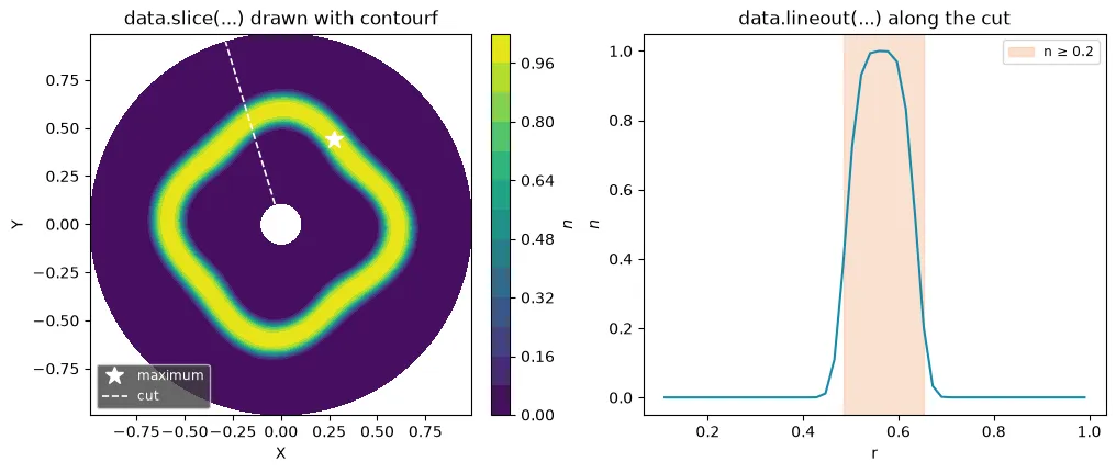## Analysis on the selection [Section titled “Analysis on the selection”](#analysis-on-the-selection) The selection is an ordinary `DataArray`, so xarray and numpy work on it directly. For the ring from the [contour-line example](/plasma-plots/guides/field-plots/#contour-lines): ```python last = n.plasma.data.slice(coords="physical", plane="XY", t=-1, eta3=0) densest = last.isel(last.argmax(...)) # the densest point, with its X and Y print(float(densest.X), float(densest.Y)) cut = n.plasma.data.lineout(x="eta1", t=-1, eta2=0.3, eta3=0) radius = 0.1 + 0.9 * cut.eta1 # this mapping's minor radius inside = radius.where(cut >= 0.2) width = float(inside.max() - inside.min()) # the ring's width along the cut # (t, eta1, eta2) frames = n.plasma.data.view(coords="physical", plane="XY", eta3=0) peak_over_time = frames.max("t") # the largest density each point reached ``` The same selections drawn with plain matplotlib: ```python fig, (ax_map, ax_cut) = plt.subplots(1, 2) ax_map.contourf(last.X, last.Y, last, levels=12) ax_map.plot(densest.X, densest.Y, "w*") ax_cut.plot(radius, cut) ax_cut.axvspan(float(inside.min()), float(inside.max()), alpha=0.25) ```  ## Exports [Section titled “Exports”](#exports) ```python last.to_dataframe() # a pandas table, one row per point, with X and Y last.to_netcdf("ring_last.nc") # a self-describing file with all coordinates np.save("ring_last.npy", last.values) # the bare numbers n.plasma.data.to_vtk("ring") # one .vts per time and a .pvd for ParaView ``` ## Other plotting libraries [Section titled “Other plotting libraries”](#other-plotting-libraries) `plasma-plots` never depends on another plotting library. The selected data goes to any of them; for Plotly there is also a shortcut, `backend="plotly"`, which draws every plot as an interactive Plotly figure (see [Interactive plots with Plotly](/plasma-plots/guides/plotly/)). Built by hand, a 2-D slice as a Plotly heatmap: ```python import plotly.express as px selected = field.plasma.data.slice(x="eta1", y="eta2", t=-1) px.imshow( selected.transpose("eta2", "eta1"), x=selected.eta1, y=selected.eta2, origin="lower", color_continuous_scale="viridis", ) ``` Loading interactive chart… # API reference > Every accessor, function and class of plasma-plots, generated from the docstrings. The reference is generated from the docstrings, so it always matches the code. The guides show the same functionality with figures. Where the accessors come from The examples use output of a Struphy `Output`, which loads plasma-plots and its `.plasma` accessors. For other xarray data, run `import plasma_plots` first (see [Getting started](/plasma-plots/guides/getting-started/#loading-plasma-plots)). ## Accessors [Section titled “Accessors”](#accessors) Most of plasma-plots is reached through accessors on the objects Struphy returns: | Accessor | What it does | | ---------------------------------------------------------------- | ------------------------------------------------------------------------------- | | [`array.plasma.plot`](/plasma-plots/reference/plot/) | Plots of one labeled array: time series, slices, animations, spectra, 3-D views | | [`array.plasma.analysis`](/plasma-plots/reference/analysis/) | Diagnostics of one labeled array: fits, norms, errors, spectra, vector calculus | | [`array.plasma.data`](/plasma-plots/reference/data/) | The selected data behind every plot, without drawing it | | [`dataset.plasma`](/plasma-plots/reference/dataset/) | Plots, diagnostics and data of marker Datasets such as orbits | | [`out.plot` and `out.analysis`](/plasma-plots/reference/output/) | Whole-run plots and diagnostics of a Struphy `Output` | A method’s page lists every parameter, including those it shares with the function it wraps. ## Modules [Section titled “Modules”](#modules) The functions behind the accessors, to call on a plain `xarray.DataArray`, and the analytic theory: | Module | Contents | | ------------------------------------------------------------------------------- | ----------------------------------------------------------------------------------------------------------------------------------------------------------------------------- | | [`plasma_plots.plotting`](/plasma-plots/api/plasma_plots/plotting/) | Plotting functions for labeled Struphy output | | [`plasma_plots.analysis`](/plasma-plots/api/plasma_plots/analysis/) | Numerical diagnostics: fits, norms, errors, integrals, vector calculus, orbits | | [`plasma_plots.spectral`](/plasma-plots/api/plasma_plots/spectral/) | Fourier transforms, filters, peaks, mode spectra, matrix pencil | | [`plasma_plots.spectral_plots`](/plasma-plots/api/plasma_plots/spectral_plots/) | Plots of spectra, filters, modes and fits | | [`plasma_plots.pyvista_plots`](/plasma-plots/api/plasma_plots/pyvista_plots/) | Three-dimensional PyVista views and VTK export | | [`plasma_plots.arrays`](/plasma-plots/api/plasma_plots/arrays/) | Labels, validation and helpers for labeled arrays | | [`plasma_plots.theory`](/plasma-plots/api/plasma_plots/theory/) | Analytic theory: kinetic, wave, orbit, exact-solution and numerics results (see the [Theory guide](/plasma-plots/guides/theory/)) | | [`plasma_plots.plotly_backend`](/plasma-plots/api/plasma_plots/plotly_backend/) | `backend="plotly"`: the conversion of Matplotlib figures into interactive Plotly figures (see [Interactive plots](/plasma-plots/guides/plotly/)) | | [`plasma_plots.tikz_backend`](/plasma-plots/api/plasma_plots/tikz_backend/) | `backend="tikz"`: the conversion into TikZ/pgfplots figures for LaTeX, by maxplotlib (see [LaTeX figures](/plasma-plots/guides/latex/)) | | [`plasma_plots.gallery`](/plasma-plots/api/plasma_plots/gallery/) | Output helpers of the [example gallery](https://struphy-hub.github.io/examples/): Plotly figure files, profiling exports and metadata (`pip install "plasma-plots[gallery]"`) | The full module tree is under **All modules** in the sidebar. For other tools, each package also has an `objects.inv` (for Sphinx and mkdocstrings links) and an `llms.txt` at [`/api/plasma_plots/`](/plasma-plots/api/plasma_plots/). # array.plasma.analysis > Diagnostics of one labeled array: fits, norms, errors, spectra, vector calculus. Numerical diagnostics of one labeled `xarray.DataArray`, as `array.plasma.analysis.(...)`. They return labeled arrays and Datasets, so their results can be plotted with `.plasma.plot` in turn. Where the accessors come from The examples use output of a Struphy `Output`, which loads plasma-plots and its `.plasma` accessors. For other xarray data, run `import plasma_plots` first (see [Getting started](/plasma-plots/guides/getting-started/#loading-plasma-plots)). ## array.plasma.analysis [Section titled “array.plasma.analysis”](#arrayplasmaanalysis) Quantitative diagnostics of one array, as `array.plasma.analysis.(...)`. ### `growth_rate` [Section titled “growth\_rate”](#growth_rate) ### `growth_rate`method[#](#plasma_plots.accessors.ArrayAnalysis.growth_rate) [View source](https://github.com/max-models/plasma-plots/blob/devel/src/plasma_plots/accessors.py#L3041-L3079 "src/plasma_plots/accessors.py:3041-3079") ``` def growth_rate(window: tuple[float | None, float | None] = (None, None), amplitude: bool = False) ``` Fit `exp(rate * t + intercept)` to this time series within `window`. Parameters | Name | Type | Default | Description | | ----------- | -------------------------------- | -------------- | -------------------------------------------------------------------------------------------------------- | | `window` | `(float or None, float or None)` | `(None, None)` | The time interval `(t0, t1)` of the fitted samples; `None` for an open end. Default: every sample. | | `amplitude` | `bool` | `False` | The series is quadratic in an amplitude (e.g. an energy): return the amplitude’s rate. Default: `False`. | Returns * `FitResult or None` `.rate`, `.intercept`, `.time` and `.fitted`; `None` with fewer than two valid samples. See Also [`plasma_plots.analysis.growth_rate()`](/plasma-plots/api/plasma_plots/analysis/#plasma_plots.analysis.growth_rate) : The function behind this method. [`ArrayAnalysis.damping_rate()`](/plasma-plots/api/plasma_plots/accessors/#plasma_plots.accessors.ArrayAnalysis.damping_rate) : The same fit to the envelope of an oscillating series. [`ArrayPlots.timeseries()`](/plasma-plots/api/plasma_plots/accessors/#plasma_plots.accessors.ArrayPlots.timeseries) : The series with the fit drawn (`fit=`). Examples ```python >>> energy.plasma.analysis.growth_rate(window=(0.0, 5.0), amplitude=True).rate ``` ### `damping_rate` [Section titled “damping\_rate”](#damping_rate) ### `damping_rate`method[#](#plasma_plots.accessors.ArrayAnalysis.damping_rate) [View source](https://github.com/max-models/plasma-plots/blob/devel/src/plasma_plots/accessors.py#L3081-L3119 "src/plasma_plots/accessors.py:3081-3119") ``` def damping_rate(window: tuple[float | None, float | None] = (None, None), amplitude: bool = False) ``` Fit exponential decay to the envelope of this oscillating time series. Parameters | Name | Type | Default | Description | | ----------- | -------------------------------- | -------------- | -------------------------------------------------------------------------------------------------------- | | `window` | `(float or None, float or None)` | `(None, None)` | The time interval `(t0, t1)` of the peaks that are used; `None` for an open end. Default: every sample. | | `amplitude` | `bool` | `False` | The series is quadratic in an amplitude (e.g. an energy): return the amplitude’s rate. Default: `False`. | Returns * `FitResult or None` The fit to the peaks; the rate is negative for damping. `None` with fewer than two valid peaks. See Also [`plasma_plots.analysis.damping_rate()`](/plasma-plots/api/plasma_plots/analysis/#plasma_plots.analysis.damping_rate) : The function behind this method. [`ArrayAnalysis.growth_rate()`](/plasma-plots/api/plasma_plots/accessors/#plasma_plots.accessors.ArrayAnalysis.growth_rate) : The same fit to the series itself. [`ArrayAnalysis.envelope()`](/plasma-plots/api/plasma_plots/accessors/#plasma_plots.accessors.ArrayAnalysis.envelope) : The peaks that are fitted. Examples ```python >>> energy.plasma.analysis.damping_rate(amplitude=True).rate ``` ### `oscillation_frequency` [Section titled “oscillation\_frequency”](#oscillation_frequency) ### `oscillation_frequency`method[#](#plasma_plots.accessors.ArrayAnalysis.oscillation_frequency) [View source](https://github.com/max-models/plasma-plots/blob/devel/src/plasma_plots/accessors.py#L3121-L3149 "src/plasma_plots/accessors.py:3121-3149") ``` def oscillation_frequency(window: tuple[float | None, float | None] = (None, None), method: str = 'zero_crossings', detrend: bool = True) ``` Measure the frequency of this oscillating time series from its zero crossings or peaks. Parameters | Name | Type | Default | Description | | --------- | -------------------------------- | ------------------ | ----------------------------------------------------------------------------------------------------------------------------------------------------------------------------------------------------------------------------- | | `window` | `(float or None, float or None)` | `(None, None)` | The time interval `(t0, t1)` used; `None` for an open end. Default: every sample. | | `method` | `('zero_crossings', 'peaks')` | `"zero_crossings"` | Count the crossings of the mean (half a period apart), or the maxima (a period apart; for a signal that does not cross its mean, e.g. an energy, whose peaks are half the field’s period apart). Default: `"zero_crossings"`. | | `detrend` | `bool` | `True` | Subtract the mean over the window first, so that crossings are of the mean. Default: `True`. | Returns * `OscillationFit or None` `omega`, `period` and the `times` of the crossings or peaks used; `None` with fewer than two. See Also [`plasma_plots.analysis.oscillation_frequency()`](/plasma-plots/api/plasma_plots/analysis/#plasma_plots.analysis.oscillation_frequency) : The function behind this method. [`ArrayAnalysis.damping_rate()`](/plasma-plots/api/plasma_plots/accessors/#plasma_plots.accessors.ArrayAnalysis.damping_rate) : The decay of the same oscillation. Examples ```python >>> probe.plasma.analysis.oscillation_frequency(window=(5.0, 40.0)).omega ``` ### `map_coordinate` [Section titled “map\_coordinate”](#map_coordinate) ### `map_coordinate`method[#](#plasma_plots.accessors.ArrayAnalysis.map_coordinate) [View source](https://github.com/max-models/plasma-plots/blob/devel/src/plasma_plots/accessors.py#L3151-L3182 "src/plasma_plots/accessors.py:3151-3182") ``` def map_coordinate(dim: str, mapping, *, name: str | None = None, units: str | None = None, label: str | None = None) -> xr.DataArray ``` Replace a coordinate by a function of it, e.g. `eta1` by the minor radius in meters. Parameters | Name | Type | Default | Description | | --------- | ------------------- | -------- | --------------------------------------------------------------------------------------------------------------------- | | `dim` | `str` | required | The dimension whose coordinate is mapped, e.g. `"eta1"`. | | `mapping` | `callable or float` | required | A function of the coordinate’s values (`lambda eta1: 0.1 + 0.9 * eta1`), or a factor (a length, for `length * eta1`). | | `name` | `str` | `None` | The name of the new dimension, e.g. `"r"`. Default: keep `dim`. | | `units` | `str` | `None` | The new coordinate’s units, e.g. `"m"`. Default: none. | | `label` | `str` | `None` | The new coordinate’s axis label (its `long_name`), mathtext allowed. Default: `name`. | Returns * `xarray.DataArray` The array over the new coordinate, which every plot then draws and labels. See Also [`plasma_plots.arrays.map_coordinate()`](/plasma-plots/api/plasma_plots/arrays/#plasma_plots.arrays.map_coordinate) : The function behind this method. Examples ```python >>> r_T = T.plasma.analysis.map_coordinate( ... "eta1", lambda eta1: 0.1 + 0.9 * eta1, name="r", units="m" ... ) >>> r_T.plasma.plot.profiles(x="r", eta2=0, eta3=0) ``` ### `envelope` [Section titled “envelope”](#envelope) ### `envelope`method[#](#plasma_plots.accessors.ArrayAnalysis.envelope) [View source](https://github.com/max-models/plasma-plots/blob/devel/src/plasma_plots/accessors.py#L3184-L3198 "src/plasma_plots/accessors.py:3184-3198") ``` def envelope() -> xr.DataArray ``` Return the local maxima of this time series. Returns * `xarray.DataArray` The peaks, over their times `t`. See Also [`plasma_plots.analysis.envelope()`](/plasma-plots/api/plasma_plots/analysis/#plasma_plots.analysis.envelope) : The function behind this method. ### `norm` [Section titled “norm”](#norm) ### `norm`method[#](#plasma_plots.accessors.ArrayAnalysis.norm) [View source](https://github.com/max-models/plasma-plots/blob/devel/src/plasma_plots/accessors.py#L3200-L3218 "src/plasma_plots/accessors.py:3200-3218") ``` def norm(dims=None, squared: bool = False) -> xr.DataArray ``` Return the L2 norm over `dims` (default: every dimension except `t`). Parameters | Name | Type | Default | Description | | --------- | ------------------------ | ------- | ---------------------------------------------------------------- | | `dims` | `str or sequence of str` | `None` | The dimensions summed over. Default: every dimension except `t`. | | `squared` | `bool` | `False` | Return the squared norm `Σ f²` instead. Default: `False`. | Returns * `xarray.DataArray` The norm over the remaining dimensions, e.g. `t`. See Also [`plasma_plots.analysis.norm()`](/plasma-plots/api/plasma_plots/analysis/#plasma_plots.analysis.norm) : The function behind this method. Examples ```python >>> div_B.plasma.analysis.norm() ``` ### `drift` [Section titled “drift”](#drift) ### `drift`method[#](#plasma_plots.accessors.ArrayAnalysis.drift) [View source](https://github.com/max-models/plasma-plots/blob/devel/src/plasma_plots/accessors.py#L3220-L3239 "src/plasma_plots/accessors.py:3220-3239") ``` def drift(ref=None) -> xr.DataArray ``` Return the signed deviation of this time series from `ref` or from its first sample. Parameters | Name | Type | Default | Description | | ----- | ----------------------------------------- | ------- | ---------------------------------------------------------------------------------- | | `ref` | `float or array_like or xarray.DataArray` | `None` | The reference, broadcast against `data`. Default: `data` at the first time sample. | Returns * `xarray.DataArray` The deviation over `t`. See Also [`plasma_plots.analysis.drift()`](/plasma-plots/api/plasma_plots/analysis/#plasma_plots.analysis.drift) : The function behind this method. [`ArrayAnalysis.relative_error()`](/plasma-plots/api/plasma_plots/accessors/#plasma_plots.accessors.ArrayAnalysis.relative_error) : The absolute relative deviation. Examples ```python >>> energy.plasma.analysis.drift().plasma.plot.timeseries() ``` ### `relative_error` [Section titled “relative\_error”](#relative_error) ### `relative_error`method[#](#plasma_plots.accessors.ArrayAnalysis.relative_error) [View source](https://github.com/max-models/plasma-plots/blob/devel/src/plasma_plots/accessors.py#L3241-L3260 "src/plasma_plots/accessors.py:3241-3260") ``` def relative_error(ref=None, skip_first: bool = True) -> xr.DataArray ``` Return the absolute relative deviation from `ref` or from this series’ first sample. Parameters | Name | Type | Default | Description | | ------------ | ----------------------------------------- | ------- | --------------------------------------------------------------------------------------------------------------- | | `ref` | `float or array_like or xarray.DataArray` | `None` | The reference, broadcast against `data`; must be non-zero everywhere. Default: `data` at the first time sample. | | `skip_first` | `bool` | `True` | Leave out the first time sample (zero against the default reference). Default: `True`. | Returns * `xarray.DataArray` The relative deviation over `t`. See Also [`plasma_plots.analysis.relative_error()`](/plasma-plots/api/plasma_plots/analysis/#plasma_plots.analysis.relative_error) : The function behind this method. [`ArrayAnalysis.drift()`](/plasma-plots/api/plasma_plots/accessors/#plasma_plots.accessors.ArrayAnalysis.drift) : The signed deviation. Examples ```python >>> energy.plasma.analysis.relative_error(ref=exact_solution) ``` ### `spatial_average` [Section titled “spatial\_average”](#spatial_average) ### `spatial_average`method[#](#plasma_plots.accessors.ArrayAnalysis.spatial_average) [View source](https://github.com/max-models/plasma-plots/blob/devel/src/plasma_plots/accessors.py#L3262-L3282 "src/plasma_plots/accessors.py:3262-3282") ``` def spatial_average(dims=None) -> xr.DataArray ``` Return the mean over the logical space dimensions `eta1`, `eta2`, `eta3` (or `dims`). For a binned `e1_v1` distribution this is f(v1, t) averaged over space. Parameters | Name | Type | Default | Description | | ------ | ------------------------ | ------- | ------------------------------------------------------------------------------------------------------------------------------------------ | | `dims` | `str or sequence of str` | `None` | The dimensions averaged over. Default: every logical dimension (`eta1`, `eta2`, `eta3`, or GVEC’s `rho`, `theta`, `zeta`) that `data` has. | Returns * `xarray.DataArray` The mean over the remaining dimensions. See Also [`plasma_plots.analysis.spatial_average()`](/plasma-plots/api/plasma_plots/analysis/#plasma_plots.analysis.spatial_average) : The function behind this method. Examples ```python >>> distribution.plasma.analysis.spatial_average() ``` ### `velocity_moments` [Section titled “velocity\_moments”](#velocity_moments) ### `velocity_moments`method[#](#plasma_plots.accessors.ArrayAnalysis.velocity_moments) [View source](https://github.com/max-models/plasma-plots/blob/devel/src/plasma_plots/accessors.py#L3284-L3304 "src/plasma_plots/accessors.py:3284-3304") ``` def velocity_moments(dims=None) -> xr.Dataset ``` Return density, mean velocity and variance of a binned distribution over its velocity dimensions. See [`plasma_plots.analysis.velocity_moments()`](/plasma-plots/api/plasma_plots/analysis/#plasma_plots.analysis.velocity_moments) for the definitions. Parameters | Name | Type | Default | Description | | ------ | ------------------------ | ------- | ------------------------------------------------------------------------------------------------------------------------------------------ | | `dims` | `str or sequence of str` | `None` | The velocity dimensions integrated over, each with a coordinate of at least two bins. Default: every one of `v1`, `v2`, `v3` that `f` has. | Returns * `xarray.Dataset` The moments, over the remaining dimensions. See Also [`plasma_plots.analysis.velocity_moments()`](/plasma-plots/api/plasma_plots/analysis/#plasma_plots.analysis.velocity_moments) : The function behind this method. Examples ```python >>> distribution.plasma.analysis.velocity_moments() ``` ### `dispersion` [Section titled “dispersion”](#dispersion) ### `dispersion`method[#](#plasma_plots.accessors.ArrayAnalysis.dispersion) [View source](https://github.com/max-models/plasma-plots/blob/devel/src/plasma_plots/accessors.py#L3306-L3334 "src/plasma_plots/accessors.py:3306-3334") ``` def dispersion(dim: str | None = None, detrend: bool = True) -> xr.DataArray ``` Return the space-time power spectrum of this `(t, dim)` field. A plain FFT, as a function of angular frequency and wavenumber: the data behind a dispersion-relation plot ([`ArrayPlots.dispersion()`](/plasma-plots/api/plasma_plots/accessors/#plasma_plots.accessors.ArrayPlots.dispersion)). `dim` defaults to the sole dimension other than `t`; select every other dimension away first. `omega` comes out in the angular-frequency units implied by `t`’s spacing (e.g. rad/s for physical seconds, or a normalized angular frequency for normalized time). Parameters | Name | Type | Default | Description | | --------- | ------ | ------- | --------------------------------------------------------------------------------------------------------------------------------------------- | | `dim` | `str` | `None` | The spatial dimension. Default: the sole dimension other than `t`. | | `detrend` | `bool` | `True` | Remove the time-mean at each point of `dim` first, which otherwise dominates the spectrum as a spurious zero-frequency line. Default: `True`. | Returns * `xarray.DataArray` The power over `omega` and the wavenumber. See Also [`plasma_plots.analysis.power_spectrum()`](/plasma-plots/api/plasma_plots/analysis/#plasma_plots.analysis.power_spectrum) : The function behind this method, and the definition. [`ArrayPlots.dispersion()`](/plasma-plots/api/plasma_plots/accessors/#plasma_plots.accessors.ArrayPlots.dispersion) : The plot of this spectrum. [`ArrayAnalysis.fit_branches()`](/plasma-plots/api/plasma_plots/accessors/#plasma_plots.accessors.ArrayAnalysis.fit_branches) : Straight branches fitted to it. Examples ```python >>> spectrum = E.isel(eta2=0, eta3=0).plasma.analysis.dispersion() ``` ### `fit_branches` [Section titled “fit\_branches”](#fit_branches) ### `fit_branches`method[#](#plasma_plots.accessors.ArrayAnalysis.fit_branches) [View source](https://github.com/max-models/plasma-plots/blob/devel/src/plasma_plots/accessors.py#L3336-L3371 "src/plasma_plots/accessors.py:3336-3371") ``` def fit_branches(n_branches: int, k_range: tuple[float, float] | None = None, noise_level: float = 0.5, order: int = 10) ``` Fit straight dispersion branches (`omega = v * k`) to this `(omega, k)` power spectrum. Parameters | Name | Type | Default | Description | | ------------- | ---------------- | -------- | ----------------------------------------------------------------------------------------------------------------------------------------------------------------------------------------------------------- | | `n_branches` | `int` | required | The number of branches, at least 1. | | `k_range` | `(float, float)` | `None` | The interval of non-negative k’s that are scanned. Default: `(k.max() / 8, k.max() / 2)`, which in practice skips both the low-k region where branches have not yet separated, and the folded Nyquist edge. | | `noise_level` | `float` | `0.5` | Maxima count only above this fraction of the column’s peak power. Default: 0.5. | | `order` | `int` | `10` | A local maximum must exceed every one of its `order` neighbors on both sides along omega (out-of-range neighbors are clipped to the edge sample, as in `scipy.signal.argrelextrema`). Default: 10. | Returns * `list of BranchFit` One fit per branch. See Also [`plasma_plots.analysis.fit_dispersion_branches()`](/plasma-plots/api/plasma_plots/analysis/#plasma_plots.analysis.fit_dispersion_branches) : The function behind this method. [`ArrayAnalysis.dispersion()`](/plasma-plots/api/plasma_plots/accessors/#plasma_plots.accessors.ArrayAnalysis.dispersion) : The spectrum to fit. [`ArrayAnalysis.trace_branch()`](/plasma-plots/api/plasma_plots/accessors/#plasma_plots.accessors.ArrayAnalysis.trace_branch) : The measured frequency along a curved branch. Examples ```python >>> field.plasma.analysis.dispersion().plasma.analysis.fit_branches( ... n_branches=2 ... ) ``` ### `fft` [Section titled “fft”](#fft) ### `fft`method[#](#plasma_plots.accessors.ArrayAnalysis.fft) [View source](https://github.com/max-models/plasma-plots/blob/devel/src/plasma_plots/accessors.py#L3375-L3396 "src/plasma_plots/accessors.py:3375-3396") ``` def fft(dim: str, detrend: bool = False, window: str | None = None) -> xr.DataArray ``` Return the two-sided Fourier coefficients along `dim`. Parameters | Name | Type | Default | Description | | --------- | ---------------- | -------- | ------------------------------------------------------------------------------------------ | | `dim` | `str` | required | The dimension to transform. | | `detrend` | `bool` | `False` | Subtract the mean along `dim` first. Default: False. | | `window` | `(None, 'hann')` | `None` | Multiply by a periodic Hann window (see \[`hann()`]\[hann]) first. Default: None (boxcar). | Returns * `xarray.DataArray` The complex coefficients. See Also [`plasma_plots.spectral.fft()`](/plasma-plots/api/plasma_plots/spectral/#plasma_plots.spectral.fft) : The function behind this method. [`ArrayAnalysis.time_fft()`](/plasma-plots/api/plasma_plots/accessors/#plasma_plots.accessors.ArrayAnalysis.time_fft) : The one-sided transform in time. Examples ```python >>> phi.plasma.analysis.fft(dim="eta1") ``` ### `time_fft` [Section titled “time\_fft”](#time_fft) ### `time_fft`method[#](#plasma_plots.accessors.ArrayAnalysis.time_fft) [View source](https://github.com/max-models/plasma-plots/blob/devel/src/plasma_plots/accessors.py#L3398-L3419 "src/plasma_plots/accessors.py:3398-3419") ``` def time_fft(detrend: bool = False, window: str | None = None) -> xr.Dataset ``` Return the one-sided temporal coefficients and the power per bin. Parameters | Name | Type | Default | Description | | --------- | ---------------- | ------- | ------------------------------------------------------------------------------------------ | | `detrend` | `bool` | `False` | Subtract the temporal mean first. Default: False. | | `window` | `(None, 'hann')` | `None` | Multiply by a periodic Hann window (see \[`hann()`]\[hann]) first. Default: None (boxcar). | Returns * `xarray.Dataset` `coefficients` and `power` over `omega` and the other dimensions. See Also [`plasma_plots.spectral.time_fft()`](/plasma-plots/api/plasma_plots/spectral/#plasma_plots.spectral.time_fft) : The function behind this method. [`ArrayPlots.power_spectrum()`](/plasma-plots/api/plasma_plots/accessors/#plasma_plots.accessors.ArrayPlots.power_spectrum) : The plot of the power. Examples ```python >>> phi.plasma.analysis.time_fft(detrend=True) ``` ### `filter_time` [Section titled “filter\_time”](#filter_time) ### `filter_time`method[#](#plasma_plots.accessors.ArrayAnalysis.filter_time) [View source](https://github.com/max-models/plasma-plots/blob/devel/src/plasma_plots/accessors.py#L3421-L3442 "src/plasma_plots/accessors.py:3421-3442") ``` def filter_time(dims=None, omega_min: float = 1e-08, pad_bins: int = 0) ``` Return the dominant frequency band, reconstructed. Parameters | Name | Type | Default | Description | | ----------- | ------------------------ | ------- | ------------------------------------------------------------------------------------------------------------------------------------------------------------------------------- | | `dims` | `str or sequence of str` | `None` | Non-time dimensions to sum the power over before choosing the band. Default: all dimensions except `t` and `component`. Pass `dims=()` for independent filtering at each point. | | `omega_min` | `float` | `1e-08` | Finite, positive lowest frequency considered, which excludes DC. Default: 1e-8. | | `pad_bins` | `int` | `0` | Nonnegative number of extra bins on each side of the band. Default: 0. | Returns * `TimeFilterResult` The band and the reconstructed signal. See Also [`plasma_plots.spectral.filter_time()`](/plasma-plots/api/plasma_plots/spectral/#plasma_plots.spectral.filter_time) : The function behind this method. [`ArrayPlots.filtered()`](/plasma-plots/api/plasma_plots/accessors/#plasma_plots.accessors.ArrayPlots.filtered) : A probe of the signal against the reconstruction. Examples ```python >>> band = phi.plasma.analysis.filter_time(dims=("eta1", "eta2", "eta3")) ``` ### `band_filter` [Section titled “band\_filter”](#band_filter) ### `band_filter`method[#](#plasma_plots.accessors.ArrayAnalysis.band_filter) [View source](https://github.com/max-models/plasma-plots/blob/devel/src/plasma_plots/accessors.py#L3444-L3465 "src/plasma_plots/accessors.py:3444-3465") ``` def band_filter(omega_lo: float, omega_hi: float, *, detrend: bool = False) -> xr.DataArray ``` Return only the frequencies in `[omega_lo, omega_hi]`. Parameters | Name | Type | Default | Description | | ---------- | ------- | -------- | ------------------------------------------------------------------------------------------------------------- | | `omega_lo` | `float` | required | The lowest angular frequency kept. | | `omega_hi` | `float` | required | The highest angular frequency kept, at least `omega_lo`. | | `detrend` | `bool` | `False` | Subtract the temporal mean first; the result then has zero mean even if the band includes DC. Default: False. | Returns * `xarray.DataArray` The filtered signal, on this array’s grid. See Also [`plasma_plots.spectral.band_filter()`](/plasma-plots/api/plasma_plots/spectral/#plasma_plots.spectral.band_filter) : The function behind this method. [`ArrayAnalysis.filter_time()`](/plasma-plots/api/plasma_plots/accessors/#plasma_plots.accessors.ArrayAnalysis.filter_time) : The dominant band, found automatically. Examples ```python >>> phi.plasma.analysis.band_filter(0.08, 0.11) ``` ### `spectral_peaks` [Section titled “spectral\_peaks”](#spectral_peaks) ### `spectral_peaks`method[#](#plasma_plots.accessors.ArrayAnalysis.spectral_peaks) [View source](https://github.com/max-models/plasma-plots/blob/devel/src/plasma_plots/accessors.py#L3467-L3501 "src/plasma_plots/accessors.py:3467-3501") ``` def spectral_peaks(n_peaks: int = 3, dims=None, omega_min: float = 1e-08, detrend=True, window=None) -> xr.Dataset ``` Return the strongest spectral peaks, with sub-bin frequencies. Parameters | Name | Type | Default | Description | | ----------- | ------------------------ | ------- | ----------------------------------------------------------------------------------------------------------------------------------------------------------------------------------------------------------------------------------------------------------------------------------------------------------------------------------------------------- | | `n_peaks` | `int` | `3` | The number of peaks to return at most. Default: 3. | | `dims` | `str or sequence of str` | `None` | Dimensions to sum the power over. Default: every dimension but `omega`. Only `omega` may remain. | | `omega_min` | `float` | `1e-08` | The lowest frequency a peak may have, which excludes DC. Default: 1e-8. | | `detrend` | `bool or int` | `True` | For a time series: `True` subtracts the mean, `False` nothing, and an integer is the degree of a least-squares polynomial in `t` removed at every point first. An energy such as LinearMHD’s `en_U` oscillates at twice the wave frequency around a slow trend, so its peaks with `detrend=2` sit at `2 * omega`. Ignored for spectra. Default: True. | | `window` | `(None, 'hann')` | `None` | Window applied before transforming a time series. Default: None. | Returns * `xarray.Dataset` The peaks, strongest first. See Also [`plasma_plots.spectral.spectral_peaks()`](/plasma-plots/api/plasma_plots/spectral/#plasma_plots.spectral.spectral_peaks) : The function behind this method. [`ArrayPlots.power_spectrum()`](/plasma-plots/api/plasma_plots/accessors/#plasma_plots.accessors.ArrayPlots.power_spectrum) : The spectrum with the peaks labeled (`peaks=`). Examples ```python >>> phi.plasma.analysis.spectral_peaks(n_peaks=2) ``` ### `spectrogram` [Section titled “spectrogram”](#spectrogram) ### `spectrogram`method[#](#plasma_plots.accessors.ArrayAnalysis.spectrogram) [View source](https://github.com/max-models/plasma-plots/blob/devel/src/plasma_plots/accessors.py#L3503-L3526 "src/plasma_plots/accessors.py:3503-3526") ``` def spectrogram(length, step=None, detrend: bool = True, window: str | None = 'hann') -> xr.DataArray ``` Return power spectra in sliding time windows. Parameters | Name | Type | Default | Description | | --------- | ---------------- | -------- | ----------------------------------------------------------------------------------------------------------- | | `length` | `int or float` | required | The window length: a sample count (integer, 4 to the number of samples) or a time span (float). | | `step` | `int or float` | `None` | The shift between windows: a sample count (integer) or a time span (float). Default: a quarter of `length`. | | `detrend` | `bool` | `True` | Subtract each window’s mean. Default: True. | | `window` | `('hann', None)` | `"hann"` | The taper of each window, not compensated for. Default: `"hann"`. | Returns * `xarray.DataArray` The power over `(t, omega, ...)`, `t` being each window’s center. See Also [`plasma_plots.spectral.spectrogram()`](/plasma-plots/api/plasma_plots/spectral/#plasma_plots.spectral.spectrogram) : The function behind this method. [`ArrayPlots.spectrogram()`](/plasma-plots/api/plasma_plots/accessors/#plasma_plots.accessors.ArrayPlots.spectrogram) : The plot of these spectra. Examples ```python >>> signal.plasma.analysis.spectrogram(length=200.0, step=10.0) ``` ### `mode_spectrum` [Section titled “mode\_spectrum”](#mode_spectrum) ### `mode_spectrum`method[#](#plasma_plots.accessors.ArrayAnalysis.mode_spectrum) [View source](https://github.com/max-models/plasma-plots/blob/devel/src/plasma_plots/accessors.py#L3528-L3551 "src/plasma_plots/accessors.py:3528-3551") ``` def mode_spectrum(dims=None, names=('m', 'n'), periods=None, scale=None) -> xr.DataArray ``` Return the complex amplitudes over poloidal/toroidal mode numbers. Parameters | Name | Type | Default | Description | | --------- | ---------------------------- | ------------ | ---------------------------------------------------------------------------------------------------------------------------------------------------------------------------------------------------------------------------------------------------------------------------------------------- | | `dims` | `str or sequence of str` | `None` | The periodic dimensions to transform. Default: the two angles of the logical dimensions (see [`plasma_plots.arrays.logical_dims()`](/plasma-plots/api/plasma_plots/arrays/#plasma_plots.arrays.logical_dims)), `("eta2", "eta3")` for Struphy. | | `names` | `str or sequence of str` | `('m', 'n')` | The name of the mode number of each dimension, one per dimension. Default: `("m", "n")`. | | `periods` | `float or sequence of float` | `None` | Each direction’s period in its coordinate: one number for all, or one per dimension. Default: the coordinate’s `period` attribute (see [`plasma_plots.arrays.angle_period()`](/plasma-plots/api/plasma_plots/arrays/#plasma_plots.arrays.angle_period)), else 1.0. | | `scale` | `int or sequence of int` | `None` | Multiplies the mode numbers (one number, or one per dimension; cast to integers), e.g. `scale=(1, 6)` labels a sixth of a torus (Struphy’s `tor_period=6`) with full-torus toroidal mode numbers. Default: 2π over the `period` attribute of an angle (nfp for GVEC’s toroidal angle), else 1. | Returns * `xarray.DataArray` The amplitudes over the mode numbers `names` and every remaining dimension. See Also [`plasma_plots.spectral.mode_spectrum()`](/plasma-plots/api/plasma_plots/spectral/#plasma_plots.spectral.mode_spectrum) : The function behind this method. [`ArrayAnalysis.mode_amplitudes()`](/plasma-plots/api/plasma_plots/accessors/#plasma_plots.accessors.ArrayAnalysis.mode_amplitudes) : Real amplitudes of this spectrum. Examples ```python >>> modes = phi.plasma.analysis.mode_spectrum() ``` ### `mode_amplitudes` [Section titled “mode\_amplitudes”](#mode_amplitudes) ### `mode_amplitudes`method[#](#plasma_plots.accessors.ArrayAnalysis.mode_amplitudes) [View source](https://github.com/max-models/plasma-plots/blob/devel/src/plasma_plots/accessors.py#L3553-L3574 "src/plasma_plots/accessors.py:3553-3574") ``` def mode_amplitudes(top: int | None = None, real: bool = True, relative: bool = False) -> xr.DataArray ``` Return the real amplitudes of this mode spectrum along one `mode` dimension. Parameters | Name | Type | Default | Description | | ---------- | ------ | ------- | ------------------------------------------------------------------------------------------------------------------------------------------------------------------------------------------------------------------------------------------------------------------------------------------------------------------------------- | | `top` | `int` | `None` | Keep only the `top` modes with the largest peak amplitude over every other dimension, strongest first. Default: all modes. | | `real` | `bool` | `True` | The field is real: each `(m, n)` is combined with its conjugate `(-m, -n)`. Only the half with the first nonzero mode number positive is kept, and its amplitude doubled, so a field `A cos(...)` gives `A`. A mode without a twin on the grid (the mean, or the Nyquist mode of an even grid) is kept as it is. Default: True. | | `relative` | `bool` | `False` | Divide by the amplitude of the mean (the mode with all numbers zero), which is then left out: e.g. density perturbations relative to the background density, as growth plots of an instability often show. NaN where the mean vanishes. Default: False. | Returns * `xarray.DataArray` The amplitudes over `mode` and every remaining dimension. See Also [`plasma_plots.spectral.mode_amplitudes()`](/plasma-plots/api/plasma_plots/spectral/#plasma_plots.spectral.mode_amplitudes) : The function behind this method. [`ArrayAnalysis.mode_spectrum()`](/plasma-plots/api/plasma_plots/accessors/#plasma_plots.accessors.ArrayAnalysis.mode_spectrum) : The spectrum this is applied to. Examples ```python >>> phi.plasma.analysis.mode_spectrum().plasma.analysis.mode_amplitudes(top=4) ``` ### `mode_structure` [Section titled “mode\_structure”](#mode_structure) ### `mode_structure`method[#](#plasma_plots.accessors.ArrayAnalysis.mode_structure) [View source](https://github.com/max-models/plasma-plots/blob/devel/src/plasma_plots/accessors.py#L3576-L3597 "src/plasma_plots/accessors.py:3576-3597") ``` def mode_structure(omega: float, *, window: str | None = 'hann', detrend: bool = True) -> xr.DataArray ``` Return the complex amplitude at the exact frequency `omega` at every point. Parameters | Name | Type | Default | Description | | --------- | ---------------- | -------- | --------------------------------------------------------------------------------------------- | | `omega` | `float` | required | The angular frequency ω. | | `window` | `('hann', None)` | `"hann"` | The weights `w(t)`: a periodic Hann window, or `None` for uniform weights. Default: `"hann"`. | | `detrend` | `bool` | `True` | Subtract the temporal mean at every point first. Default: True. | Returns * `xarray.DataArray` The complex amplitude over every dimension but `t`. See Also [`plasma_plots.spectral.mode_structure()`](/plasma-plots/api/plasma_plots/spectral/#plasma_plots.spectral.mode_structure) : The function behind this method. [`ArrayPlots.mode_profiles()`](/plasma-plots/api/plasma_plots/accessors/#plasma_plots.accessors.ArrayPlots.mode_profiles) : The harmonics of this eigenfunction (`omega=`). Examples ```python >>> phi.plasma.analysis.mode_structure(omega) ``` ### `cross_spectrum` [Section titled “cross\_spectrum”](#cross_spectrum) ### `cross_spectrum`method[#](#plasma_plots.accessors.ArrayAnalysis.cross_spectrum) [View source](https://github.com/max-models/plasma-plots/blob/devel/src/plasma_plots/accessors.py#L3599-L3627 "src/plasma_plots/accessors.py:3599-3627") ``` def cross_spectrum(other: xr.DataArray, *, dims=None, detrend: bool = True, window=None) -> xr.Dataset ``` Return the cross-spectrum, phase (of `other` relative to this) and coherence. Parameters | Name | Type | Default | Description | | --------- | ------------------------ | -------- | ------------------------------------------------------------------------------------------ | | `other` | `xarray.DataArray` | required | The second signal, on the same time grid; its phase is relative to this one. | | `dims` | `str or sequence of str` | `None` | Dimensions to sum the cross-spectrum over, as an ensemble. Default: none (no `coherence`). | | `detrend` | `bool` | `True` | Subtract each signal’s temporal mean first. Default: True. | | `window` | `(None, 'hann')` | `None` | Window applied to both signals before transforming. Default: None. | Returns * `xarray.Dataset` The cross-spectrum, phase and (with `dims`) coherence over `omega`. See Also [`plasma_plots.spectral.cross_spectrum()`](/plasma-plots/api/plasma_plots/spectral/#plasma_plots.spectral.cross_spectrum) : The function behind this method. [`ArrayPlots.cross_spectrum()`](/plasma-plots/api/plasma_plots/accessors/#plasma_plots.accessors.ArrayPlots.cross_spectrum) : The plot of this spectrum. Examples ```python >>> u.plasma.analysis.cross_spectrum(b, dims="eta3") ``` ### `matrix_pencil` [Section titled “matrix\_pencil”](#matrix_pencil) ### `matrix_pencil`method[#](#plasma_plots.accessors.ArrayAnalysis.matrix_pencil) [View source](https://github.com/max-models/plasma-plots/blob/devel/src/plasma_plots/accessors.py#L3629-L3652 "src/plasma_plots/accessors.py:3629-3652") ``` def matrix_pencil(n_modes: int = 1, pencil: int | None = None, detrend: bool = False) -> xr.Dataset ``` Return frequencies and growth rates beyond the FFT resolution. Parameters | Name | Type | Default | Description | | --------- | ------ | ------- | ------------------------------------------------------------------------------------------------------------------------------------------------------------------------------ | | `n_modes` | `int` | `1` | The number of modes to fit and return: real oscillations for a real signal, complex exponentials for a complex one. The fit needs well over `2 * n_modes` samples. Default: 1. | | `pencil` | `int` | `None` | The pencil parameter (Hankel matrix width minus one), which trades noise robustness against resolution. Default: `N // 2`. | | `detrend` | `bool` | `False` | Subtract the mean first. Default: False. | Returns * `xarray.Dataset` `omega`, `gamma`, `amplitude` and `phase` along `mode`, strongest first. See Also [`plasma_plots.spectral.matrix_pencil()`](/plasma-plots/api/plasma_plots/spectral/#plasma_plots.spectral.matrix_pencil) : The function behind this method. [`ArrayPlots.pencil_fit()`](/plasma-plots/api/plasma_plots/accessors/#plasma_plots.accessors.ArrayPlots.pencil_fit) : The plot of this fit. Examples ```python >>> probe.plasma.analysis.matrix_pencil(n_modes=1) ``` ### `gradient` [Section titled “gradient”](#gradient) ### `gradient`method[#](#plasma_plots.accessors.ArrayAnalysis.gradient) [View source](https://github.com/max-models/plasma-plots/blob/devel/src/plasma_plots/accessors.py#L3654-L3672 "src/plasma_plots/accessors.py:3654-3672") ``` def gradient(domain=None) -> xr.DataArray ``` Return the Cartesian gradient of this scalar field on a mapped domain. Parameters | Name | Type | Default | Description | | -------- | ---------------- | ------- | --------------------------------------------------------------------------------------------------------------------- | | `domain` | `struphy domain` | `None` | The mapping (`out.domain`), for the exact Jacobian. Default: differentiate the `X`, `Y`, `Z` coordinates numerically. | Returns * `xarray.DataArray` The gradient, with a `component` dimension `(x, y, z)`. See Also [`plasma_plots.analysis.gradient()`](/plasma-plots/api/plasma_plots/analysis/#plasma_plots.analysis.gradient) : The function behind this method. Examples ```python >>> phi.plasma.analysis.gradient() ``` ### `surface_average` [Section titled “surface\_average”](#surface_average) ### `surface_average`method[#](#plasma_plots.accessors.ArrayAnalysis.surface_average) [View source](https://github.com/max-models/plasma-plots/blob/devel/src/plasma_plots/accessors.py#L3674-L3697 "src/plasma_plots/accessors.py:3674-3697") ``` def surface_average(jacobian=None, domain=None, quadrature=None) -> xr.DataArray ``` Return the flux-surface average of this field over its two angles. Parameters | Name | Type | Default | Description | | ------------ | ------------------ | ------- | ---------------------------------------------------------------------------------------------------------------------------------------------------------------------------------------------------- | | `jacobian` | `xarray.DataArray` | `None` | `√g` on the same grid, e.g. GVEC’s `Jac` (its absolute value is used). Default: from `domain`, else the numerical Jacobian of the `X`, `Y`, `Z` coordinates, which needs at least two radial points. | | `domain` | `struphy domain` | `None` | The mapping, for the exact `√g` of a Struphy run. | | `quadrature` | `dict` | `None` | Explicit weights for the angles, as for \[`volume_integral()`]\[volume\_integral]. | Returns * `xarray.DataArray` `⟨f⟩` over the radius and every non-spatial dimension. See Also [`plasma_plots.analysis.surface_average()`](/plasma-plots/api/plasma_plots/analysis/#plasma_plots.analysis.surface_average) : The function behind this method. [`DatasetAnalysis.surface_average()`](/plasma-plots/api/plasma_plots/accessors/#plasma_plots.accessors.DatasetAnalysis.surface_average) : The same, with the Dataset’s `Jac`. Examples ```python >>> ev.mod_B.plasma.analysis.surface_average(jacobian=ev.Jac) ``` ### `rational_surfaces` [Section titled “rational\_surfaces”](#rational_surfaces) ### `rational_surfaces`method[#](#plasma_plots.accessors.ArrayAnalysis.rational_surfaces) [View source](https://github.com/max-models/plasma-plots/blob/devel/src/plasma_plots/accessors.py#L3699-L3722 "src/plasma_plots/accessors.py:3699-3722") ``` def rational_surfaces(count: int = 4, nfp: int | None = None, max_denominator: int = 12) -> xr.DataArray ``` Return where this rotational transform (or safety factor) profile is a low-order rational. Parameters | Name | Type | Default | Description | | ----------------- | ----- | ------- | ----------------------------------------------------------------------------------------------------------------------------------------------------------------------------------------------------- | | `count` | `int` | `4` | The number of rational values. Default: 4. | | `nfp` | `int` | `None` | The numerators are multiples of it. Default: the profile’s `nfp` attribute (GVEC’s, see [`plasma_plots.gvec.from_gvec()`](/plasma-plots/api/plasma_plots/gvec/#plasma_plots.gvec.from_gvec)), else 1. | | `max_denominator` | `int` | `12` | The largest `m`. Default: 12. | Returns * `xarray.DataArray` The positions over `surface`, with the coordinates `n`, `m` and `value`. See Also [`plasma_plots.analysis.rational_surfaces()`](/plasma-plots/api/plasma_plots/analysis/#plasma_plots.analysis.rational_surfaces) : The function behind this method. [`ArrayPlots.lineout()`](/plasma-plots/api/plasma_plots/accessors/#plasma_plots.accessors.ArrayPlots.lineout) : `rationals=` marks them on the profile. Examples ```python >>> ev.iota.plasma.analysis.rational_surfaces(count=3) ``` ### `error` [Section titled “error”](#error) ### `error`method[#](#plasma_plots.accessors.ArrayAnalysis.error) [View source](https://github.com/max-models/plasma-plots/blob/devel/src/plasma_plots/accessors.py#L3724-L3762 "src/plasma_plots/accessors.py:3724-3762") ``` def error(exact, *, norm: str = 'rms', relative: bool = False, dims=None, weighted: bool = False, domain=None, args=None) -> xr.DataArray ``` Return the error against an exact solution (an array or a function of the coordinates). Parameters | Name | Type | Default | Description | | ---------- | ---------------------------------------------------- | -------- | -------------------------------------------------------------------------------------------------------------------------------------------------------------------------------------------------------------------------------------------------------------------------------------------------------------- | | `exact` | `(callable, array_like, number or xarray.DataArray)` | required | The exact solution: an array (aligned with `data`, or broadcast to it) or a function of its coordinates, evaluated with \[`evaluate_on()`]\[evaluate\_on], e.g. `lambda x, y, z, t: ...`. | | `norm` | `('rms', 'max', 'l1', 'l2', 'pointwise')` | `"rms"` | `"pointwise"` is the difference `data − exact` itself; `"max"` the largest absolute difference; `"l1"` the mean (or, weighted, the integral) of `\|data − exact\|`; `"l2"` the square root of the mean (or integral) of `\|data − exact\|²`; `"rms"` (default) as `"l2"`, divided by the volume when weighted. | | `relative` | `bool` | `False` | Divide by the same norm of the exact solution; for `"pointwise"`, by the largest `\|exact\|` over the whole array. Default: `False`. | | `dims` | `str or sequence of str` | `None` | The dimensions the norm is taken over. Default: every dimension but `t`. Weighted norms need exactly `eta1`, `eta2`, `eta3`. | | `weighted` | `bool` | `False` | Integrate over the physical volume instead of averaging over the grid points (no effect on `"max"` and `"pointwise"`). Default: `False`. | | `domain` | `struphy domain` | `None` | The mapping (`out.domain`), for the exact `\|√g\|` of weighted norms. Default: from the `X`, `Y`, `Z` coordinates. | | `args` | `sequence of str` | `None` | The coordinates passed to a callable `exact`, as in \[`evaluate_on()`]\[evaluate\_on]. Default: `X`, `Y`, `Z` (or the logical dimensions), then `t`. | Returns * `xarray.DataArray` The error, over the dimensions not reduced by `norm`. See Also [`plasma_plots.analysis.error()`](/plasma-plots/api/plasma_plots/analysis/#plasma_plots.analysis.error) : The function behind this method. Examples ```python >>> T.plasma.analysis.error(exact, relative=True) >>> T.plasma.analysis.error(exact, norm="max") ``` ### `project_mode` [Section titled “project\_mode”](#project_mode) ### `project_mode`method[#](#plasma_plots.accessors.ArrayAnalysis.project_mode) [View source](https://github.com/max-models/plasma-plots/blob/devel/src/plasma_plots/accessors.py#L3764-L3797 "src/plasma_plots/accessors.py:3764-3797") ``` def project_mode(dim: str, number: float, kind: str = 'sin', period: float = 1.0, bin_correction: bool = False) -> xr.DataArray ``` Return the amplitude of one Fourier mode along `dim`. Parameters | Name | Type | Default | Description | | ---------------- | --------------------------- | -------- | ------------------------------------------------------------------------------------------------------------------------------------------------------------------------------------------------------------------- | | `dim` | `str` | required | The periodic dimension, e.g. `"eta1"`. | | `number` | `float` | required | The mode number, not a wavenumber: `k = 2π number / L`. | | `kind` | `('sin', 'cos', 'complex')` | `"sin"` | `"sin"` (default) gives `a` of `a sin(2π number x / period)`: `2 ⟨f sin(…)⟩`; `"cos"` the cosine amplitude, and `"complex"` the complex amplitude `2 ⟨f exp(−i…)⟩` (`abs()` the amplitude, `np.angle()` the phase). | | `period` | `float` | `1.0` | The period of `dim`. Default: 1, the logical unit interval. | | `bin_correction` | `bool` | `False` | Undo the damping of binned particle data, whose bins average the mode over their width `h`: divide by `sinc(number h / period)`. Default: `False`. | Returns * `xarray.DataArray` The amplitude over the other dimensions. See Also [`plasma_plots.analysis.project_mode()`](/plasma-plots/api/plasma_plots/analysis/#plasma_plots.analysis.project_mode) : The function behind this method. Examples ```python >>> rho.plasma.analysis.project_mode(dim="eta2", number=3, kind="complex") ``` ### `divergence` [Section titled “divergence”](#divergence) ### `divergence`method[#](#plasma_plots.accessors.ArrayAnalysis.divergence) [View source](https://github.com/max-models/plasma-plots/blob/devel/src/plasma_plots/accessors.py#L3799-L3817 "src/plasma_plots/accessors.py:3799-3817") ``` def divergence(components: str = 'cartesian', domain=None) -> xr.DataArray ``` Return the divergence of this vector field. Parameters | Name | Type | Default | Description | | ------------ | -------------------------------- | ------------- | ---------------------------------------------------------------------------------------------------------------------------------------------------- | | `components` | `('cartesian', 'contravariant')` | `"cartesian"` | What the components are, as for the 3-D views: `"cartesian"` (default) `(x, y, z)`, or `"contravariant"` components, which are pushed forward first. | | `domain` | `struphy domain` | `None` | The mapping (`out.domain`), for the exact Jacobian. Default: from the `X`, `Y`, `Z` coordinates. | Returns * `xarray.DataArray` The divergence, without the `component` dimension. See Also [`plasma_plots.analysis.divergence()`](/plasma-plots/api/plasma_plots/analysis/#plasma_plots.analysis.divergence) : The function behind this method. Examples ```python >>> B.plasma.analysis.divergence() ``` ### `curl` [Section titled “curl”](#curl) ### `curl`method[#](#plasma_plots.accessors.ArrayAnalysis.curl) [View source](https://github.com/max-models/plasma-plots/blob/devel/src/plasma_plots/accessors.py#L3819-L3837 "src/plasma_plots/accessors.py:3819-3837") ``` def curl(components: str = 'cartesian', domain=None) -> xr.DataArray ``` Return the curl of this vector field, in Cartesian components. Parameters | Name | Type | Default | Description | | ------------ | -------------------------------- | ------------- | ------------------------------------------------------------------------------------------------------------------------------ | | `components` | `('cartesian', 'contravariant')` | `"cartesian"` | What the components are: `"cartesian"` (default) `(x, y, z)`, or `"contravariant"` components, which are pushed forward first. | | `domain` | `struphy domain` | `None` | The mapping (`out.domain`), for the exact Jacobian. Default: from the `X`, `Y`, `Z` coordinates. | Returns * `xarray.DataArray` The curl, with a `component` dimension. See Also [`plasma_plots.analysis.curl()`](/plasma-plots/api/plasma_plots/analysis/#plasma_plots.analysis.curl) : The function behind this method. Examples ```python >>> B.plasma.analysis.curl() ``` ### `flux_function` [Section titled “flux\_function”](#flux_function) ### `flux_function`method[#](#plasma_plots.accessors.ArrayAnalysis.flux_function) [View source](https://github.com/max-models/plasma-plots/blob/devel/src/plasma_plots/accessors.py#L3839-L3857 "src/plasma_plots/accessors.py:3839-3857") ``` def flux_function() -> xr.DataArray ``` Return the flux (or stream) function of this 2-D in-plane field. Returns * `xarray.DataArray` The flux function, without the `component` dimension. See Also [`plasma_plots.analysis.flux_function()`](/plasma-plots/api/plasma_plots/analysis/#plasma_plots.analysis.flux_function) : The function behind this method. Examples ```python >>> B.plasma.analysis.flux_function() ``` ### `cylindrical_components` [Section titled “cylindrical\_components”](#cylindrical_components) ### `cylindrical_components`method[#](#plasma_plots.accessors.ArrayAnalysis.cylindrical_components) [View source](https://github.com/max-models/plasma-plots/blob/devel/src/plasma_plots/accessors.py#L3859-L3878 "src/plasma_plots/accessors.py:3859-3878") ``` def cylindrical_components() -> xr.DataArray ``` Return the Cartesian components rotated to `(R, phi, Z)`. Returns * `xarray.DataArray` The vector field in cylindrical components. See Also [`plasma_plots.analysis.cylindrical_components()`](/plasma-plots/api/plasma_plots/analysis/#plasma_plots.analysis.cylindrical_components) : The function behind this method. [`ArrayAnalysis.toroidal_components()`](/plasma-plots/api/plasma_plots/accessors/#plasma_plots.accessors.ArrayAnalysis.toroidal_components) : Components about a magnetic axis. Examples ```python >>> E.plasma.analysis.cylindrical_components() ``` ### `toroidal_components` [Section titled “toroidal\_components”](#toroidal_components) ### `toroidal_components`method[#](#plasma_plots.accessors.ArrayAnalysis.toroidal_components) [View source](https://github.com/max-models/plasma-plots/blob/devel/src/plasma_plots/accessors.py#L3880-L3899 "src/plasma_plots/accessors.py:3880-3899") ``` def toroidal_components(R0: float, Z0: float = 0.0) -> xr.DataArray ``` Return the Cartesian components rotated to `(radial, poloidal, toroidal)` about an axis at `R0`. Parameters | Name | Type | Default | Description | | ---- | ------- | -------- | -------------------------------------------- | | `R0` | `float` | required | The major radius of the magnetic axis. | | `Z0` | `float` | `0.0` | The height of the magnetic axis. Default: 0. | Returns * `xarray.DataArray` The vector field in toroidal components. See Also [`plasma_plots.analysis.toroidal_components()`](/plasma-plots/api/plasma_plots/analysis/#plasma_plots.analysis.toroidal_components) : The function behind this method. [`ArrayAnalysis.cylindrical_components()`](/plasma-plots/api/plasma_plots/accessors/#plasma_plots.accessors.ArrayAnalysis.cylindrical_components) : Components about the `Z` axis. Examples ```python >>> u.plasma.analysis.toroidal_components(R0=3.0) ``` ### `polar_coordinates` [Section titled “polar\_coordinates”](#polar_coordinates) ### `polar_coordinates`method[#](#plasma_plots.accessors.ArrayAnalysis.polar_coordinates) [View source](https://github.com/max-models/plasma-plots/blob/devel/src/plasma_plots/accessors.py#L3901-L3919 "src/plasma_plots/accessors.py:3901-3919") ``` def polar_coordinates(center=(0.0, 0.0)) -> xr.DataArray ``` Return this array with coordinates `r` and `theta` in the `X`-`Y` plane. Parameters | Name | Type | Default | Description | | -------- | ---------------- | ------------ | -------------------------------------------------------------------- | | `center` | `(float, float)` | `(0.0, 0.0)` | The origin `(X, Y)` of the polar coordinates. Default: `(0.0, 0.0)`. | Returns * `xarray.DataArray` This array with the added coordinates. See Also [`plasma_plots.analysis.polar_coordinates()`](/plasma-plots/api/plasma_plots/analysis/#plasma_plots.analysis.polar_coordinates) : The function behind this method. Examples ```python >>> n.plasma.analysis.polar_coordinates(center=(0.0, 0.0)) ``` ### `trace_branch` [Section titled “trace\_branch”](#trace_branch) ### `trace_branch`method[#](#plasma_plots.accessors.ArrayAnalysis.trace_branch) [View source](https://github.com/max-models/plasma-plots/blob/devel/src/plasma_plots/accessors.py#L3921-L3946 "src/plasma_plots/accessors.py:3921-3946") ``` def trace_branch(theory, *, window: float = 0.2, k_range=None, threshold: float = 0.001) -> xr.Dataset ``` Return the measured frequency of a dispersion branch near `theory(k)` in this `(omega, k)` spectrum. Parameters | Name | Type | Default | Description | | ----------- | ---------------- | -------- | --------------------------------------------------------------------------------------------------------------------------------------------------------------------------------------- | | `theory` | `callable` | required | The expected branch `omega(k)`, applied to an array of `k`; of a complex frequency (as [`plasma_plots.theory`](/plasma-plots/api/plasma_plots/theory/) returns), the real part is used. | | `window` | `float` | `0.2` | The relative half-width of the search window about the theory. Default: 0.2. | | `k_range` | `(float, float)` | `None` | The `k` interval to trace (negative `k` are never traced). Default: every `k >= 0`. | | `threshold` | `float` | `0.001` | Maxima weaker than this times the strongest one found count as no wave. Default: 1e-3. | Returns * `xarray.Dataset` The measured branch over `k`. See Also [`plasma_plots.spectral.trace_branch()`](/plasma-plots/api/plasma_plots/spectral/#plasma_plots.spectral.trace_branch) : The function behind this method. [`ArrayPlots.against_theory()`](/plasma-plots/api/plasma_plots/accessors/#plasma_plots.accessors.ArrayPlots.against_theory) : The measured frequencies against the theory. Examples ```python >>> spectrum.plasma.analysis.trace_branch( ... bohm_gross, window=0.2, k_range=(1.5, 5.5) ... ) ``` ### `drop_periodic_endpoint` [Section titled “drop\_periodic\_endpoint”](#drop_periodic_endpoint) ### `drop_periodic_endpoint`method[#](#plasma_plots.accessors.ArrayAnalysis.drop_periodic_endpoint) [View source](https://github.com/max-models/plasma-plots/blob/devel/src/plasma_plots/accessors.py#L3948-L3962 "src/plasma_plots/accessors.py:3948-3962") ``` def drop_periodic_endpoint(dim: str, *, period: float = 1.0) -> xr.DataArray ``` Return this array without a duplicated periodic endpoint along `dim`. Parameters | Name | Type | Default | Description | | -------- | ------- | -------- | ---------------------------------------------------- | | `dim` | `str` | required | The periodic dimension. | | `period` | `float` | `1.0` | The period in the coordinate of `dim`. Default: 1.0. | Returns * `xarray.DataArray` This array, one point shorter along `dim` if its last point repeats the first. See Also [`plasma_plots.spectral.drop_periodic_endpoint()`](/plasma-plots/api/plasma_plots/spectral/#plasma_plots.spectral.drop_periodic_endpoint) : The function behind this method. ### `field_lines` [Section titled “field\_lines”](#field_lines) ### `field_lines`method[#](#plasma_plots.accessors.ArrayAnalysis.field_lines) [View source](https://github.com/max-models/plasma-plots/blob/devel/src/plasma_plots/accessors.py#L3964-L4022 "src/plasma_plots/accessors.py:3964-4022") ``` def field_lines(seeds=8, turns: float | None = None, length: float | None = None, step: float | None = None, direction: str = 'forward', section: float | None = None, stride: int | None = None, components: str = 'cartesian', **selection) -> xr.Dataset ``` Trace field lines of this vector field through its mapped grid. Parameters | Name | Type | Default | Description | | ------------- | ------------------------------------------- | ------------- | ----------------------------------------------------------------------------------------------------------------------------------------------------------------------------------------------------------------------------------------------------------------------------------------------------------------------------------------------------------------------------------------------------------------------------------------------------------------------------------------------------------------------------------------------------------------------------------------- | | `seeds` | `(int, dict, array_like or xarray.Dataset)` | `8` | Where the lines start, in logical coordinates: a number of seeds spread along the radial coordinate at the first poloidal and toroidal grid values (the outboard midplane of a torus whose angles start at 0); a dict of logical coordinates to values or 1-D arrays, which are combined into a grid of seeds (e.g. `{"rho": 0.95, "theta": thetas, "zeta": zetas}` for a connection-length map; a missing coordinate takes its first grid value); an `(n, 3)` array of points in the order of the logical dimensions; or a Dataset with one variable per logical coordinate. Default: 8. | | `turns` | `float` | `None` | Stop a line after this many toroidal transits (turns of the torus: nfp periods of the toroidal logical coordinate, i.e. 2π of GVEC’s toroidal angle, one period of Struphy’s `eta3`). Default: 20 when the toroidal direction wraps around, else none. | | `length` | `float` | `None` | Stop a line after this arc length, in the units of `X`, `Y`, `Z`. Default: with `turns`, 1.5 times the length `turns` circles through the seeds’ mean major radius would take (a safety net); without, four times the grid’s extent. | | `step` | `float` | `None` | The step of arc length of the integrator. Default: the median spacing of the grid points (trilinear interpolation limits the accuracy before the step does). | | `direction` | `('forward', 'backward', 'both')` | `"forward"` | Along the field, against it, or each seed in both directions (two lines per seed, with the coordinates `seed` and `direction` telling them apart; the connection length is then the sum of both). Default: `"forward"`. | | `section` | `float` | `None` | The toroidal logical coordinate of the poloidal plane whose punctures are recorded. Default: the first toroidal grid value (e.g. `zeta = 0`). | | `stride` | `int` | `None` | Save every `stride`-th step of each line. Default: as many as keep each line at about 20 000 samples at most; the punctures, transits and lengths count every step regardless. | | `components` | `('cartesian', 'contravariant')` | `"cartesian"` | What the components are: `"cartesian"` (default) `(x, y, z)`, or contravariant logical components, as for [`plasma_plots.analysis.divergence()`](/plasma-plots/api/plasma_plots/analysis/#plasma_plots.analysis.divergence). | | `**selection` | | `{}` | The other dimensions, e.g. `t=-1`: an integer is a position, a float the nearest coordinate value. | Returns * `xarray.Dataset` The lines over `(s, line)` with their punctures, rotational transforms and connection lengths; it has `.plasma.plot.poincare()`, `.footprint()` and the other field-line plots. See Also [`plasma_plots.fieldlines.trace_field_lines()`](/plasma-plots/api/plasma_plots/fieldlines/#plasma_plots.fieldlines.trace_field_lines) : The function behind this method. [`DatasetPlots.poincare()`](/plasma-plots/api/plasma_plots/accessors/#plasma_plots.accessors.DatasetPlots.poincare) : The Poincaré plot of the lines. [`ArrayAnalysis.sample_along()`](/plasma-plots/api/plasma_plots/accessors/#plasma_plots.accessors.ArrayAnalysis.sample_along) : A field along them. Examples ```python >>> lines = B.plasma.analysis.field_lines(seeds=12, turns=100, t=-1) >>> lines.plasma.plot.poincare(color_by="iota") >>> edge = B.plasma.analysis.field_lines( ... seeds={"eta1": 0.98, "eta2": np.linspace(0, 1, 32)}, ... direction="both", ... t=-1, ... ) ``` ### `sample_along` [Section titled “sample\_along”](#sample_along) ### `sample_along`method[#](#plasma_plots.accessors.ArrayAnalysis.sample_along) [View source](https://github.com/max-models/plasma-plots/blob/devel/src/plasma_plots/accessors.py#L4024-L4045 "src/plasma_plots/accessors.py:4024-4045") ``` def sample_along(lines: xr.Dataset) -> xr.DataArray ``` Return this scalar field interpolated along traced field lines. Parameters | Name | Type | Description | | ------- | ---------------- | ------------------------------------------------------------ | | `lines` | `xarray.Dataset` | The lines of \[`trace_field_lines()`]\[trace\_field\_lines]. | Returns * `xarray.DataArray` The field over `(s, line)` after its other dimensions. See Also [`plasma_plots.fieldlines.sample_along()`](/plasma-plots/api/plasma_plots/fieldlines/#plasma_plots.fieldlines.sample_along) : The function behind this method. [`ArrayAnalysis.parallel_wavenumber()`](/plasma-plots/api/plasma_plots/accessors/#plasma_plots.accessors.ArrayAnalysis.parallel_wavenumber) : The dominant wavenumber along each line. [`ArrayPlots.along_field_lines()`](/plasma-plots/api/plasma_plots/accessors/#plasma_plots.accessors.ArrayPlots.along_field_lines) : The plot. Examples ```python >>> along = phi.plasma.analysis.sample_along(lines) >>> along.isel(line=0).plasma.plot.slice(x="s", y="t") ``` ### `parallel_wavenumber` [Section titled “parallel\_wavenumber”](#parallel_wavenumber) ### `parallel_wavenumber`method[#](#plasma_plots.accessors.ArrayAnalysis.parallel_wavenumber) [View source](https://github.com/max-models/plasma-plots/blob/devel/src/plasma_plots/accessors.py#L4047-L4079 "src/plasma_plots/accessors.py:4047-4079") ``` def parallel_wavenumber(lines: xr.Dataset | None = None, method: str = 'fft', detrend: bool = True) -> xr.DataArray ``` Return the dominant parallel wavenumber of this field along field lines. Parameters | Name | Type | Default | Description | | --------- | ---------------------- | ------- | ------------------------------------------------------------------------------------------------------------------------------------------------------------------------------------------------------------------------------- | | `lines` | `xarray.Dataset` | `None` | Traced lines to sample this field along first. Default: this array already is the samples of [`sample_along()`](/plasma-plots/api/plasma_plots/accessors/#plasma_plots.accessors.ArrayAnalysis.sample_along), over `(s, line)`. | | `method` | `('fft', 'crossings')` | `"fft"` | How to estimate it. Default: `"fft"`. | | `detrend` | `bool` | `True` | Remove the mean along each line first. Default: True. | Returns * `xarray.DataArray` `k_parallel` over `line` and the other dimensions. See Also [`plasma_plots.fieldlines.parallel_wavenumber()`](/plasma-plots/api/plasma_plots/fieldlines/#plasma_plots.fieldlines.parallel_wavenumber) : The function behind this method. [`plasma_plots.theory.waves.parallel_wavenumber()`](/plasma-plots/api/plasma_plots/theory/waves/#plasma_plots.theory.waves.parallel_wavenumber) : The expected `(n + m/q)/R₀`. Examples ```python >>> phi.plasma.analysis.parallel_wavenumber(lines=lines) ``` ### `boozer_spectrum` [Section titled “boozer\_spectrum”](#boozer_spectrum) ### `boozer_spectrum`method[#](#plasma_plots.accessors.ArrayAnalysis.boozer_spectrum) [View source](https://github.com/max-models/plasma-plots/blob/devel/src/plasma_plots/accessors.py#L4081-L4103 "src/plasma_plots/accessors.py:4081-4103") ``` def boozer_spectrum(top: int | None = None, angles: str = 'boozer') -> xr.DataArray ``` Return the Boozer harmonics `B_mn` of this quantity over the radius. Parameters | Name | Type | Default | Description | | -------- | ------------------- | ---------- | -------------------------------------------------------------------------------------------------------------------------------------------------------------------- | | `top` | `int` | `None` | Keep only the `top` harmonics with the largest peak amplitude over the radius, strongest first. Default: all. | | `angles` | `('boozer', 'any')` | `"boozer"` | Require the Boozer angles `theta_B`, `zeta_B` (default), or take the harmonics in whatever angles the field has (not a Boozer spectrum then; e.g. for a comparison). | Returns * `xarray.DataArray` The real amplitudes over `mode` (with `m`, `n`) and the radius. See Also [`plasma_plots.analysis.boozer_spectrum()`](/plasma-plots/api/plasma_plots/analysis/#plasma_plots.analysis.boozer_spectrum) : The function behind this method. [`ArrayAnalysis.quasisymmetry_error()`](/plasma-plots/api/plasma_plots/accessors/#plasma_plots.accessors.ArrayAnalysis.quasisymmetry_error) : The symmetry-breaking part. [`ArrayPlots.boozer_spectrum()`](/plasma-plots/api/plasma_plots/accessors/#plasma_plots.accessors.ArrayPlots.boozer_spectrum) : The plot. Examples ```python >>> boozer.mod_B.plasma.analysis.boozer_spectrum(top=8) ``` ### `quasisymmetry_error` [Section titled “quasisymmetry\_error”](#quasisymmetry_error) ### `quasisymmetry_error`method[#](#plasma_plots.accessors.ArrayAnalysis.quasisymmetry_error) [View source](https://github.com/max-models/plasma-plots/blob/devel/src/plasma_plots/accessors.py#L4105-L4126 "src/plasma_plots/accessors.py:4105-4126") ``` def quasisymmetry_error(helicity='QA', angles: str = 'boozer') -> xr.DataArray ``` Return the quasi-symmetry error of this `|B|` on each flux surface. Parameters | Name | Type | Default | Description | | ---------- | -------------------- | ---------- | ------------------------------------------------------------------------------------------------------------------------------ | | `helicity` | `('QA', 'QP', 'QH')` | `"QA"` | The symmetry: a name, or `(M, N)` with `N` a full-torus toroidal mode number (its sign picks the handedness). Default: `"QA"`. | | `angles` | `('boozer', 'any')` | `"boozer"` | As for [`boozer_spectrum()`](/plasma-plots/api/plasma_plots/accessors/#plasma_plots.accessors.ArrayAnalysis.boozer_spectrum). | Returns * `xarray.DataArray` `f_QS` over the radius. See Also [`plasma_plots.analysis.quasisymmetry_error()`](/plasma-plots/api/plasma_plots/analysis/#plasma_plots.analysis.quasisymmetry_error) : The function behind this method. [`ArrayAnalysis.boozer_spectrum()`](/plasma-plots/api/plasma_plots/accessors/#plasma_plots.accessors.ArrayAnalysis.boozer_spectrum) : The harmonics it is computed from. Examples ```python >>> boozer.mod_B.plasma.analysis.quasisymmetry_error(helicity="QH") ``` ### `critical_points` [Section titled “critical\_points”](#critical_points) ### `critical_points`method[#](#plasma_plots.accessors.ArrayAnalysis.critical_points) [View source](https://github.com/max-models/plasma-plots/blob/devel/src/plasma_plots/accessors.py#L4128-L4148 "src/plasma_plots/accessors.py:4128-4148") ``` def critical_points(refine: bool = True) -> xr.Dataset ``` Return the O-points and X-points of this flux function (at every time). Parameters | Name | Type | Default | Description | | -------- | ------ | ------- | ------------------------------------------------------------------------------------------------ | | `refine` | `bool` | `True` | Locate the zero within the cell by Newton’s method (the cell’s centre otherwise). Default: True. | Returns * `xarray.Dataset` The points over `point` (and `t`): positions, values and kinds. See Also [`plasma_plots.analysis.critical_points()`](/plasma-plots/api/plasma_plots/analysis/#plasma_plots.analysis.critical_points) : The function behind this method. [`ArrayAnalysis.reconnected_flux()`](/plasma-plots/api/plasma_plots/accessors/#plasma_plots.accessors.ArrayAnalysis.reconnected_flux) : The flux between them over time. [`ArrayPlots.critical_points()`](/plasma-plots/api/plasma_plots/accessors/#plasma_plots.accessors.ArrayPlots.critical_points) : The plot. Examples ```python >>> B.plasma.analysis.flux_function().plasma.analysis.critical_points() ``` ### `reconnected_flux` [Section titled “reconnected\_flux”](#reconnected_flux) ### `reconnected_flux`method[#](#plasma_plots.accessors.ArrayAnalysis.reconnected_flux) [View source](https://github.com/max-models/plasma-plots/blob/devel/src/plasma_plots/accessors.py#L4150-L4176 "src/plasma_plots/accessors.py:4150-4176") ``` def reconnected_flux(relative: bool = True, o_point=None, x_point=None) -> xr.DataArray ``` Return the reconnected flux over time: this flux function between an O- and an X-point. Parameters | Name | Type | Default | Description | | ---------- | ---------------- | ------- | ------------------------------------------------------------------------------------------- | | `relative` | `bool` | `True` | Subtract the value at the first time. Default: True. | | `o_point` | `(float, float)` | `None` | The logical coordinates near which to look for the O-point. Default: the dominant island’s. | | `x_point` | `(float, float)` | `None` | The same for the X-point. | Returns * `xarray.DataArray` `ΔΨ(t)`. See Also [`plasma_plots.analysis.reconnected_flux()`](/plasma-plots/api/plasma_plots/analysis/#plasma_plots.analysis.reconnected_flux) : The function behind this method. [`ArrayAnalysis.growth_rate()`](/plasma-plots/api/plasma_plots/accessors/#plasma_plots.accessors.ArrayAnalysis.growth_rate) : Its growth rate. Examples ```python >>> A = B.plasma.analysis.flux_function() >>> A.plasma.analysis.reconnected_flux().plasma.plot.timeseries( ... fit=(10.0, 30.0) ... ) ``` # array.plasma.data > The selected data behind every plot, without drawing it. Every plot on `array.plasma.plot` has a twin here, as `array.plasma.data.(...)`, that does the same selection and returns the labeled `xarray` object instead of a figure. See the [Selecting data](/plasma-plots/guides/data/) guide. Where the accessors come from The examples use output of a Struphy `Output`, which loads plasma-plots and its `.plasma` accessors. For other xarray data, run `import plasma_plots` first (see [Getting started](/plasma-plots/guides/getting-started/#loading-plasma-plots)). ## array.plasma.data [Section titled “array.plasma.data”](#arrayplasmadata) The data behind each plot in :class:`ArrayPlots`, without rendering it. ### `lineout` [Section titled “lineout”](#lineout) ### `lineout`method[#](#plasma_plots.accessors.ArrayData.lineout) [View source](https://github.com/max-models/plasma-plots/blob/devel/src/plasma_plots/accessors.py#L2582-L2616 "src/plasma_plots/accessors.py:2582-2616") ``` def lineout(x: str | None = None, **selection) -> xr.DataArray ``` Return the 1-D profile [`ArrayPlots.lineout()`](/plasma-plots/api/plasma_plots/accessors/#plasma_plots.accessors.ArrayPlots.lineout) would plot. Parameters | Name | Type | Default | Description | | ------------- | ----- | ------- | ------------------------------------------------------------------------------------------------------- | | `x` | `str` | `None` | The dimension to keep: checked to be the only one left after `selection`. Default: whichever it is. | | `**selection` | | `{}` | The other dimensions: an integer is a position (`t=-1` the last), a float the nearest coordinate value. | Returns * `xarray.DataArray` The selected profile, over `x` only. Raises * `ValueError` If more or fewer than one dimension remains, or `x` is not the remaining one. See Also [`plasma_plots.plotting.prepare_lineout()`](/plasma-plots/api/plasma_plots/plotting/#plasma_plots.plotting.prepare_lineout) : The check behind this method. [`ArrayPlots.lineout()`](/plasma-plots/api/plasma_plots/accessors/#plasma_plots.accessors.ArrayPlots.lineout) : The plot of this profile. Examples ```python >>> n.plasma.data.lineout(x="eta1", t=-1, eta2=0.3, eta3=0) ``` ### `vector` [Section titled “vector”](#vector) ### `vector`method[#](#plasma_plots.accessors.ArrayData.vector) [View source](https://github.com/max-models/plasma-plots/blob/devel/src/plasma_plots/accessors.py#L2618-L2645 "src/plasma_plots/accessors.py:2618-2645") ``` def vector(x: str, y: str, components: tuple[int, int] = (0, 1), stride: int = 1, coordinates: Coordinates = 'logical', **selection) -> xr.DataArray ``` Return the selected, strided vector field [`ArrayPlots.vector()`](/plasma-plots/api/plasma_plots/accessors/#plasma_plots.accessors.ArrayPlots.vector) would plot. Parameters | Name | Type | Default | Description | | ------------- | ------------------------- | ----------- | ------------------------------------------------------------------------------------------------------------------------------------------------------------------------------------------------------ | | `x` | `str` | required | The dimension along the horizontal axis. | | `y` | `str` | required | The dimension along the vertical axis. | | `components` | `(int, int)` | `(0, 1)` | The positions along `component_dim` of the two components drawn. Default: `(0, 1)`. | | `stride` | `int` | `1` | Draw every `stride`-th arrow along `x` and `y`. Default: `1`. | | `coordinates` | `('logical', 'physical')` | `"logical"` | Place the arrows at the logical coordinates, or at the attached physical `X`, `Y`, `Z` (then `x` and `y` must be two of `eta1`, `eta2`, `eta3`, and the axes have equal scales). Default: `"logical"`. | | `**selection` | | `{}` | Every dimension but `x`, `y` and the component dimension, e.g. `t=-1, eta3=0`: an integer is a position, a float the nearest coordinate value. | Returns * `xarray.DataArray` The two selected components over `x` and `y`, every `stride`-th point. See Also [`ArrayPlots.vector()`](/plasma-plots/api/plasma_plots/accessors/#plasma_plots.accessors.ArrayPlots.vector) : The plot of these components. [`plasma_plots.plotting.prepare_vector()`](/plasma-plots/api/plasma_plots/plotting/#plasma_plots.plotting.prepare_vector) : The function that prepares them. ### `volume_slices` [Section titled “volume\_slices”](#volume_slices) ### `volume_slices`method[#](#plasma_plots.accessors.ArrayData.volume_slices) [View source](https://github.com/max-models/plasma-plots/blob/devel/src/plasma_plots/accessors.py#L2647-L2665 "src/plasma_plots/accessors.py:2647-2665") ``` def volume_slices(indices: dict[str, int] | None = None, **selection) -> dict[str, xr.DataArray] ``` Return the three orthogonal planes [`ArrayPlots.volume_slices()`](/plasma-plots/api/plasma_plots/accessors/#plasma_plots.accessors.ArrayPlots.volume_slices) would plot. Parameters | Name | Type | Default | Description | | ------------- | -------------------- | ------- | ------------------------------------------------------------------------------------------------------------------------- | | `indices` | `dict of str to int` | `None` | The index at which each dimension is held fixed, e.g. `{"eta3": 0}`. Default: the middle index of every dimension. | | `**selection` | | `{}` | Every dimension but the three of the volume, e.g. `t=-1`: an integer is a position, a float the nearest coordinate value. | Returns * `dict of str to xarray.DataArray` The three planes. See Also [`ArrayPlots.volume_slices()`](/plasma-plots/api/plasma_plots/accessors/#plasma_plots.accessors.ArrayPlots.volume_slices) : The plot of these planes. [`plasma_plots.plotting.prepare_volume_slices()`](/plasma-plots/api/plasma_plots/plotting/#plasma_plots.plotting.prepare_volume_slices) : The function that prepares them. ### `grid` [Section titled “grid”](#grid) ### `grid`method[#](#plasma_plots.accessors.ArrayData.grid) [View source](https://github.com/max-models/plasma-plots/blob/devel/src/plasma_plots/accessors.py#L2667-L2697 "src/plasma_plots/accessors.py:2667-2697") ``` def grid(name: str | None = None, **selection) ``` Return this field as a `pyvista.StructuredGrid` on its physical points. Every dimension but `eta1`, `eta2`, `eta3` (and `component`) is selected first. This is the data behind every 3-D view, ready for any PyVista filter. Parameters | Name | Type | Default | Description | | ------------- | ----- | ------- | ---------------------------------------------------------------------------------------------------------------------------------------- | | `name` | `str` | `None` | The name of the point data. Default: the field’s label. | | `**selection` | | `{}` | Every dimension but `eta1`, `eta2`, `eta3` and `component`, e.g. `t=-1`: an integer is a position, a float the nearest coordinate value. | Returns * `pyvista.StructuredGrid` The grid, with the field as its point data. See Also [`plasma_plots.pyvista_plots.structured_grid()`](/plasma-plots/api/plasma_plots/pyvista_plots/#plasma_plots.pyvista_plots.structured_grid) : The function behind this method. [`ArrayData.to_vtk()`](/plasma-plots/api/plasma_plots/accessors/#plasma_plots.accessors.ArrayData.to_vtk) : Write the grid to files instead. Examples ```python >>> grid = phi.plasma.data.grid(t=-1) ``` ### `to_vtk` [Section titled “to\_vtk”](#to_vtk) ### `to_vtk`method[#](#plasma_plots.accessors.ArrayData.to_vtk) [View source](https://github.com/max-models/plasma-plots/blob/devel/src/plasma_plots/accessors.py#L2699-L2730 "src/plasma_plots/accessors.py:2699-2730") ``` def to_vtk(path, *, name: str | None = None, **selection) -> list[str] ``` Write this field to VTK structured-grid files for ParaView. One `.vts` per time and a `.pvd` collection, or a single `.vts` without `t`. Select other dimensions first. Parameters | Name | Type | Default | Description | | ------------- | --------------------- | -------- | ----------------------------------------------------------------------------------------------------------------------------------------------------------------- | | `path` | `str or pathlib.Path` | required | The `.vts` file (the suffix is set to `.vts`), or with a `t` dimension the directory to write into (created if needed). | | `name` | `str` | `None` | The name of the point data, also the file stem in a time series. Default: the field’s label. | | `**selection` | | `{}` | Every dimension but `t`, `eta1`, `eta2`, `eta3` and `component`: an integer is a position, a float the nearest coordinate value. `t` is kept unless selected too. | Returns * `list of str` The paths of the written files. See Also [`plasma_plots.pyvista_plots.save_vtk()`](/plasma-plots/api/plasma_plots/pyvista_plots/#plasma_plots.pyvista_plots.save_vtk) : The function behind this method. [`ArrayData.grid()`](/plasma-plots/api/plasma_plots/accessors/#plasma_plots.accessors.ArrayData.grid) : One time as a PyVista grid, in memory. Examples ```python >>> field.plasma.data.to_vtk("frames") ``` ### `slices_3d` [Section titled “slices\_3d”](#slices_3d) ### `slices_3d`method[#](#plasma_plots.accessors.ArrayData.slices_3d) [View source](https://github.com/max-models/plasma-plots/blob/devel/src/plasma_plots/accessors.py#L2732-L2749 "src/plasma_plots/accessors.py:2732-2749") ``` def slices_3d(cuts: dict | None = None, **selection) -> list[xr.DataArray] ``` Return the logical cuts [`ArrayPlots.slices_3d()`](/plasma-plots/api/plasma_plots/accessors/#plasma_plots.accessors.ArrayPlots.slices_3d) would draw. Parameters | Name | Type | Default | Description | | ------------- | ------ | ------- | ----------------------------------------------------------------------------------------------------------------------------------------------------------------------------------------------------------------------------------- | | `cuts` | `dict` | `None` | `{dim: position or list of positions}` along `eta1`, `eta2`, `eta3`: a float is the nearest logical coordinate, an integer a grid index (`-1` the last). Default: the middle of every dimension, or the whole plane of a 2-D field. | | `**selection` | | `{}` | Every dimension but `eta1`, `eta2`, `eta3`, e.g. `t=0`: an integer is a position, a float the nearest coordinate value. | Returns * `list of xarray.DataArray` One array per cut. See Also [`ArrayPlots.slices_3d()`](/plasma-plots/api/plasma_plots/accessors/#plasma_plots.accessors.ArrayPlots.slices_3d) : The drawing of these cuts. [`plasma_plots.pyvista_plots.prepare_slices_3d()`](/plasma-plots/api/plasma_plots/pyvista_plots/#plasma_plots.pyvista_plots.prepare_slices_3d) : The function that prepares them. ### `compare` [Section titled “compare”](#compare) ### `compare`method[#](#plasma_plots.accessors.ArrayData.compare) [View source](https://github.com/max-models/plasma-plots/blob/devel/src/plasma_plots/accessors.py#L2751-L2775 "src/plasma_plots/accessors.py:2751-2775") ``` def compare(other: xr.DataArray, *, mode: Literal['difference', 'ratio'] = 'difference') -> xr.DataArray ``` Return the aligned difference or ratio [`ArrayPlots.compare()`](/plasma-plots/api/plasma_plots/accessors/#plasma_plots.accessors.ArrayPlots.compare) would plot. Parameters | Name | Type | Default | Description | | ------- | ------------------------- | -------------- | -------------------------------------------------------------------------------------------- | | `other` | `xarray.DataArray` | required | The array to compare with, e.g. a reference run; aligned with this one first. | | `mode` | `('difference', 'ratio')` | `"difference"` | `first - second`, or `first / second` (NaN where `second` is zero). Default: `"difference"`. | Returns * `xarray.DataArray` This array minus `other`, or divided by it, after alignment. See Also [`ArrayPlots.compare()`](/plasma-plots/api/plasma_plots/accessors/#plasma_plots.accessors.ArrayPlots.compare) : The plot of this difference or ratio. [`plasma_plots.plotting.prepare_compare()`](/plasma-plots/api/plasma_plots/plotting/#plasma_plots.plotting.prepare_compare) : The function that computes it. Examples ```python >>> field.plasma.data.compare(reference_field, mode="ratio") ``` ### `view` [Section titled “view”](#view) ### `view`method[#](#plasma_plots.accessors.ArrayData.view) [View source](https://github.com/max-models/plasma-plots/blob/devel/src/plasma_plots/accessors.py#L2777-L2816 "src/plasma_plots/accessors.py:2777-2816") ``` def view(x: str | None = None, y: str | None = None, sweep: str = 't', coords: Coordinates = 'logical', plane: Plane = 'XY', **selection) -> xr.DataArray ``` Return every remaining dimension of this array, sweep included. This data is shared by [`ArrayPlots.panels()`](/plasma-plots/api/plasma_plots/accessors/#plasma_plots.accessors.ArrayPlots.panels), `.viewer()`, `.animation()` and `.frames()`, which each render one frame of exactly this data at a time. Parameters | Name | Type | Default | Description | | ------------- | ---------------------------------- | ----------- | ----------------------------------------------------------------------------------------------------------------------------------------------------------------------------------------- | | `x` | `str` | `None` | The dimension along the horizontal axis (logical coordinates). Default: the first of the two remaining dimensions. | | `y` | `str` | `None` | The dimension along the vertical axis. Default: the second remaining dimension. | | `sweep` | `str` | `'t'` | The dimension stepped through by panels, the viewer’s slider, animations and exported frames. Default: `"t"`. | | `coords` | `('logical', 'physical')` | `"logical"` | Draw over the logical coordinates, or over the mapped physical coordinates (`X`, `Y`, `Z`). Default: `"logical"`. | | `plane` | `('XY', 'XZ', 'YZ', 'RZ', 'X1X2')` | `"XY"` | The physical plane, with `coords="physical"`: `"RZ"` uses `R = √(X² + Y²)`, `"X1X2"` GVEC’s reference coordinates. Default: `"XY"`. | | `**selection` | | `{}` | Every dimension but `x`, `y` and `sweep`: an integer is a position (`-1` the last), a float the nearest coordinate value. Checked now; a name that is not a dimension raises `TypeError`. | Returns * `xarray.DataArray` The selection ordered `(sweep, x, y)`. With `coords="physical"` the periodic seam of a cell-centered grid is closed, as in every drawn frame (one more point along a periodic angle). Raises * `ValueError` If other dimensions than `sweep`, `x` and `y` remain, or the physical coordinates are missing. See Also [`ArrayPlots.view()`](/plasma-plots/api/plasma_plots/accessors/#plasma_plots.accessors.ArrayPlots.view) : The configured view of this data, and its options. Examples ```python >>> n.plasma.data.view(coords="physical", plane="XY", eta3=0) ``` ### `slice` [Section titled “slice”](#slice) ### `slice`method[#](#plasma_plots.accessors.ArrayData.slice) [View source](https://github.com/max-models/plasma-plots/blob/devel/src/plasma_plots/accessors.py#L2818-L2848 "src/plasma_plots/accessors.py:2818-2848") ``` def slice(x: str | None = None, y: str | None = None, sweep: str = 't', coords: Coordinates = 'logical', plane: Plane = 'XY', **selection) -> xr.DataArray ``` Return the single 2-D slice [`ArrayPlots.slice()`](/plasma-plots/api/plasma_plots/accessors/#plasma_plots.accessors.ArrayPlots.slice) would plot. Parameters | Name | Type | Default | Description | | ------------- | ---------------------------------- | ----------- | ----------------------------------------------------------------------------------------------------------------------------------------------------------------------------------------- | | `x` | `str` | `None` | The dimension along the horizontal axis (logical coordinates). Default: the first of the two remaining dimensions. | | `y` | `str` | `None` | The dimension along the vertical axis. Default: the second remaining dimension. | | `sweep` | `str` | `'t'` | The dimension stepped through by panels, the viewer’s slider, animations and exported frames. Default: `"t"`. | | `coords` | `('logical', 'physical')` | `"logical"` | Draw over the logical coordinates, or over the mapped physical coordinates (`X`, `Y`, `Z`). Default: `"logical"`. | | `plane` | `('XY', 'XZ', 'YZ', 'RZ', 'X1X2')` | `"XY"` | The physical plane, with `coords="physical"`: `"RZ"` uses `R = √(X² + Y²)`, `"X1X2"` GVEC’s reference coordinates. Default: `"XY"`. | | `**selection` | | `{}` | Every dimension but `x`, `y` and `sweep`: an integer is a position (`-1` the last), a float the nearest coordinate value. Checked now; a name that is not a dimension raises `TypeError`. | Returns * `xarray.DataArray` The selected slice. See Also [`ArrayPlots.slice()`](/plasma-plots/api/plasma_plots/accessors/#plasma_plots.accessors.ArrayPlots.slice) : The plot of this slice. Examples ```python >>> phi.plasma.data.slice(x="eta1", y="eta2", t=-1) >>> n.plasma.data.slice(coords="physical", plane="XY", t=-1, eta3=0) ``` ### `dispersion` [Section titled “dispersion”](#dispersion) ### `dispersion`method[#](#plasma_plots.accessors.ArrayData.dispersion) [View source](https://github.com/max-models/plasma-plots/blob/devel/src/plasma_plots/accessors.py#L2850-L2875 "src/plasma_plots/accessors.py:2850-2875") ``` def dispersion(dim: str | None = None, detrend: bool = True) -> xr.DataArray ``` Return the space-time power spectrum [`ArrayPlots.dispersion()`](/plasma-plots/api/plasma_plots/accessors/#plasma_plots.accessors.ArrayPlots.dispersion) would plot. The same as [`ArrayAnalysis.dispersion()`](/plasma-plots/api/plasma_plots/accessors/#plasma_plots.accessors.ArrayAnalysis.dispersion); included here too for parity with every other plot. Parameters | Name | Type | Default | Description | | --------- | ------ | ------- | --------------------------------------------------------------------------------------------------------------------------------------------- | | `dim` | `str` | `None` | The spatial dimension. Default: the sole dimension other than `t`. | | `detrend` | `bool` | `True` | Remove the time-mean at each point of `dim` first, which otherwise dominates the spectrum as a spurious zero-frequency line. Default: `True`. | Returns * `xarray.DataArray` The power over angular frequency `omega` and wavenumber. See Also [`plasma_plots.analysis.power_spectrum()`](/plasma-plots/api/plasma_plots/analysis/#plasma_plots.analysis.power_spectrum) : The function behind this method. [`ArrayPlots.dispersion()`](/plasma-plots/api/plasma_plots/accessors/#plasma_plots.accessors.ArrayPlots.dispersion) : The plot of this spectrum. [`ArrayAnalysis.dispersion()`](/plasma-plots/api/plasma_plots/accessors/#plasma_plots.accessors.ArrayAnalysis.dispersion) : The same spectrum. Examples ```python >>> field.plasma.data.dispersion(dim="eta1") ``` ### `overlay_orbits` [Section titled “overlay\_orbits”](#overlay_orbits) ### `overlay_orbits`method[#](#plasma_plots.accessors.ArrayData.overlay_orbits) [View source](https://github.com/max-models/plasma-plots/blob/devel/src/plasma_plots/accessors.py#L2877-L2905 "src/plasma_plots/accessors.py:2877-2905") ``` def overlay_orbits(orbits: xr.Dataset, *, x: str, y: str, max_markers: int = 200, **selection) -> tuple[xr.DataArray, xr.Dataset] ``` Return the field slice and marker subset [`ArrayPlots.overlay_orbits()`](/plasma-plots/api/plasma_plots/accessors/#plasma_plots.accessors.ArrayPlots.overlay_orbits) would plot. Parameters | Name | Type | Default | Description | | ------------- | ---------------- | -------- | --------------------------------------------------------------------------------------------------------------------------------------------------------------------------------------- | | `orbits` | `xarray.Dataset` | required | An orbits product with position variables named after `view.x` and `view.y` (e.g. its logical coordinates, to overlay directly on a logical-coordinates slice). | | `x` | `str` | required | The horizontal dimension of the slice. `orbits` must have a position variable of the same name (e.g. logical `eta1`, to overlay directly on a logical-coordinates slice of this field). | | `y` | `str` | required | The vertical dimension of the slice; `orbits` needs a variable of this name too. | | `max_markers` | `int` | `200` | Draw only the first `max_markers` markers. Default: `200`. | | `**selection` | | `{}` | Every other dimension of this field, e.g. `t=-1`: an integer is a position, a float the nearest coordinate value. | Returns * `tuple of (xarray.DataArray, xarray.Dataset)` The field slice, and the orbits of the first `max_markers` markers. Raises * `ValueError` If `orbits` has no variables named `x` and `y`, or no `marker` dimension. See Also [`ArrayPlots.overlay_orbits()`](/plasma-plots/api/plasma_plots/accessors/#plasma_plots.accessors.ArrayPlots.overlay_orbits) : The plot of this slice and these orbits. Examples ```python >>> field, paths = field.plasma.data.overlay_orbits( ... orbits, x="eta1", y="eta2", t=-1 ... ) ``` ### `trajectories` [Section titled “trajectories”](#trajectories) ### `trajectories`method[#](#plasma_plots.accessors.ArrayData.trajectories) [View source](https://github.com/max-models/plasma-plots/blob/devel/src/plasma_plots/accessors.py#L2907-L2928 "src/plasma_plots/accessors.py:2907-2928") ``` def trajectories(max_markers: int = 200) -> xr.Dataset ``` Return the marker-position subset [`ArrayPlots.trajectories()`](/plasma-plots/api/plasma_plots/accessors/#plasma_plots.accessors.ArrayPlots.trajectories) would plot. Parameters | Name | Type | Default | Description | | ------------- | ----- | ------- | ---------------------------------------------------------- | | `max_markers` | `int` | `200` | Draw only the first `max_markers` markers. Default: `200`. | Returns * `xarray.Dataset` The orbits of the first `max_markers` markers. Raises * `ValueError` If the orbits lack `x`, `y` or `z`, or a `marker` dimension. See Also [`ArrayPlots.trajectories()`](/plasma-plots/api/plasma_plots/accessors/#plasma_plots.accessors.ArrayPlots.trajectories) : The plot of these markers. ### `timeseries` [Section titled “timeseries”](#timeseries) ### `timeseries`method[#](#plasma_plots.accessors.ArrayData.timeseries) [View source](https://github.com/max-models/plasma-plots/blob/devel/src/plasma_plots/accessors.py#L2930-L2956 "src/plasma_plots/accessors.py:2930-2956") ``` def timeseries(*others) -> list[xr.DataArray] ``` Return this time series and any `others`, validated, as [`ArrayPlots.timeseries()`](/plasma-plots/api/plasma_plots/accessors/#plasma_plots.accessors.ArrayPlots.timeseries) plots them. Parameters | Name | Default | Description | | --------- | ------- | ---------------------------------------------------------------------------------------------------------------------- | | `*others` | `()` | Further arrays with the single dimension `t`; they may come from other runs and need not share this array’s time grid. | Returns * `list of xarray.DataArray` This series first, then `others`. Raises * `ValueError` If a series does not have the dimension `t`. See Also [`ArrayPlots.timeseries()`](/plasma-plots/api/plasma_plots/accessors/#plasma_plots.accessors.ArrayPlots.timeseries) : The plot of these series. Examples ```python >>> energy.plasma.data.timeseries(other_run_energy) ``` ### `poincare` [Section titled “poincare”](#poincare) ### `poincare`method[#](#plasma_plots.accessors.ArrayData.poincare) [View source](https://github.com/max-models/plasma-plots/blob/devel/src/plasma_plots/accessors.py#L2958-L2997 "src/plasma_plots/accessors.py:2958-2997") ``` def poincare(seeds=8, turns: float | None = None, section: float | None = None, **selection) -> xr.Dataset ``` Return the Poincaré section [`ArrayPlots.poincare()`](/plasma-plots/api/plasma_plots/accessors/#plasma_plots.accessors.ArrayPlots.poincare) would plot. Parameters | Name | Type | Default | Description | | ------------- | ------------------------------------------- | ------- | ---------------------------------------------------------------------------------------------------------------------------------------------------------------------------------------------- | | `seeds` | `(int, dict, array_like or xarray.Dataset)` | `8` | Where the lines start; see [`plasma_plots.fieldlines.trace_field_lines()`](/plasma-plots/api/plasma_plots/fieldlines/#plasma_plots.fieldlines.trace_field_lines). Default: 8 along the radius. | | `turns` | `float` | `None` | How many toroidal transits to trace. Default: 20. | | `section` | `float` | `None` | The toroidal logical coordinate of the plane. Default: the first grid value. | | `**selection` | | `{}` | The other dimensions, e.g. `t=-1`: an integer is a position, a float the nearest coordinate value. | Returns * `xarray.Dataset` The punctures over `(puncture, line)`; see [`plasma_plots.fieldlines.poincare_section()`](/plasma-plots/api/plasma_plots/fieldlines/#plasma_plots.fieldlines.poincare_section). See Also [`ArrayPlots.poincare()`](/plasma-plots/api/plasma_plots/accessors/#plasma_plots.accessors.ArrayPlots.poincare) : The plot of these punctures. [`ArrayAnalysis.field_lines()`](/plasma-plots/api/plasma_plots/accessors/#plasma_plots.accessors.ArrayAnalysis.field_lines) : The traced lines themselves. Examples ```python >>> B.plasma.data.poincare(seeds=12, turns=100, t=-1) ``` ### `critical_points` [Section titled “critical\_points”](#critical_points) ### `critical_points`method[#](#plasma_plots.accessors.ArrayData.critical_points) [View source](https://github.com/max-models/plasma-plots/blob/devel/src/plasma_plots/accessors.py#L2999-L3026 "src/plasma_plots/accessors.py:2999-3026") ``` def critical_points(refine: bool = True, **selection) -> xr.Dataset ``` Return the O- and X-points [`ArrayPlots.critical_points()`](/plasma-plots/api/plasma_plots/accessors/#plasma_plots.accessors.ArrayPlots.critical_points) would mark. Parameters | Name | Type | Default | Description | | ------------- | ------ | ------- | -------------------------------------------------------------------------------------------------- | | `refine` | `bool` | `True` | Locate the zero within the cell by Newton’s method (the cell’s centre otherwise). Default: True. | | `**selection` | | `{}` | The other dimensions, e.g. `t=-1`: an integer is a position, a float the nearest coordinate value. | Returns * `xarray.Dataset` The points over `point` (and the dimensions left, e.g. `t`). See Also [`plasma_plots.analysis.critical_points()`](/plasma-plots/api/plasma_plots/analysis/#plasma_plots.analysis.critical_points) : The function behind this method. [`ArrayPlots.critical_points()`](/plasma-plots/api/plasma_plots/accessors/#plasma_plots.accessors.ArrayPlots.critical_points) : The plot of these points. Examples ```python >>> A.plasma.data.critical_points(t=-1) ``` # dataset.plasma > Plots, diagnostics and data of marker Datasets such as orbits. Plots, diagnostics and data of an `xarray.Dataset` with per-marker variables, such as an orbits product. Where the accessors come from The examples use output of a Struphy `Output`, which loads plasma-plots and its `.plasma` accessors. For other xarray data, run `import plasma_plots` first (see [Getting started](/plasma-plots/guides/getting-started/#loading-plasma-plots)). ## dataset.plasma.plot [Section titled “dataset.plasma.plot”](#datasetplasmaplot) Plots of one dataset, as `dataset.plasma.plot.(...)`. ### `power_spectrum` [Section titled “power\_spectrum”](#power_spectrum) ### `power_spectrum`method[#](#plasma_plots.accessors.DatasetPlots.power_spectrum) [View source](https://github.com/max-models/plasma-plots/blob/devel/src/plasma_plots/accessors.py#L4586-L4620 "src/plasma_plots/accessors.py:4586-4620") ``` def power_spectrum(backend: Backend | None = None, **options) ``` Plot the power of a `time_fft` Dataset. Parameters | Name | Type | Default | Description | | ----------- | ---------------------------------- | -------------- | ---------------------------------------------------------------------------------------------------------------------------------------------------------------------------------------------------------------------------------------------------------------------------------------------------------------------------------------------------------------------------------------------------------------------------------------------------------------------------------------------- | | `**options` | | `{}` | The keyword options of [`plasma_plots.spectral_plots.plot_power_spectrum()`](/plasma-plots/api/plasma_plots/spectral_plots/#plasma_plots.spectral_plots.plot_power_spectrum), e.g. `peaks=2`. | | `backend` | `('matplotlib', 'plotly', 'tikz')` | `"matplotlib"` | Draw with Matplotlib, as an interactive Plotly figure, or as TikZ/pgfplots code for LaTeX (in `result.fig`; needs plotly or maxplotlib, see [`plasma_plots.plotly_backend`](/plasma-plots/api/plasma_plots/plotly_backend/) and [`plasma_plots.tikz_backend`](/plasma-plots/api/plasma_plots/tikz_backend/)). Default: the one set with [`plasma_plots.set_backend()`](/plasma-plots/api/plasma_plots/plotly_backend/#plasma_plots.plotly_backend.set_backend), `"matplotlib"` unless changed. | Returns * `PlotResult` The figure, the axes and the drawn artists; `data` holds the averaged `"power"` and the found `"peaks"`. See Also [`plasma_plots.spectral_plots.plot_power_spectrum()`](/plasma-plots/api/plasma_plots/spectral_plots/#plasma_plots.spectral_plots.plot_power_spectrum) : The function behind this method. [`ArrayAnalysis.time_fft()`](/plasma-plots/api/plasma_plots/accessors/#plasma_plots.accessors.ArrayAnalysis.time_fft) : The Dataset to plot. Examples ```python >>> phi.plasma.analysis.time_fft(detrend=True).plasma.plot.power_spectrum( ... peaks=2 ... ) ``` ### `cross_spectrum` [Section titled “cross\_spectrum”](#cross_spectrum) ### `cross_spectrum`method[#](#plasma_plots.accessors.DatasetPlots.cross_spectrum) [View source](https://github.com/max-models/plasma-plots/blob/devel/src/plasma_plots/accessors.py#L4622-L4655 "src/plasma_plots/accessors.py:4622-4655") ``` def cross_spectrum(omega_max: float | None = None, backend: Backend | None = None) ``` Plot the magnitude, coherence and phase of a `cross_spectrum` Dataset. Parameters | Name | Type | Default | Description | | ----------- | ---------------------------------- | -------------- | ---------------------------------------------------------------------------------------------------------------------------------------------------------------------------------------------------------------------------------------------------------------------------------------------------------------------------------------------------------------------------------------------------------------------------------------------------------------------------------------------- | | `omega_max` | `float` | `None` | The highest frequency shown. Default: all. | | `backend` | `('matplotlib', 'plotly', 'tikz')` | `"matplotlib"` | Draw with Matplotlib, as an interactive Plotly figure, or as TikZ/pgfplots code for LaTeX (in `result.fig`; needs plotly or maxplotlib, see [`plasma_plots.plotly_backend`](/plasma-plots/api/plasma_plots/plotly_backend/) and [`plasma_plots.tikz_backend`](/plasma-plots/api/plasma_plots/tikz_backend/)). Default: the one set with [`plasma_plots.set_backend()`](/plasma-plots/api/plasma_plots/plotly_backend/#plasma_plots.plotly_backend.set_backend), `"matplotlib"` unless changed. | Returns * `PlotResult` The figure, the axes and the drawn artists; `data` holds `"peak_omega"` and `"peak_phase_deg"`. See Also [`plasma_plots.spectral_plots.plot_cross_spectrum()`](/plasma-plots/api/plasma_plots/spectral_plots/#plasma_plots.spectral_plots.plot_cross_spectrum) : The function behind this method. [`ArrayAnalysis.cross_spectrum()`](/plasma-plots/api/plasma_plots/accessors/#plasma_plots.accessors.ArrayAnalysis.cross_spectrum) : The Dataset to plot. Examples ```python >>> u.plasma.analysis.cross_spectrum( ... b, dims="eta3" ... ).plasma.plot.cross_spectrum(omega_max=1.5) ``` ### `trajectories` [Section titled “trajectories”](#trajectories) ### `trajectories`method[#](#plasma_plots.accessors.DatasetPlots.trajectories) [View source](https://github.com/max-models/plasma-plots/blob/devel/src/plasma_plots/accessors.py#L4657-L4695 "src/plasma_plots/accessors.py:4657-4695") ``` def trajectories(max_markers: int = 200, show_paths: bool | None = None, ax=None, backend: Backend | None = None) ``` Plot the three-dimensional paths of saved markers, for an `orbits` product. Parameters | Name | Type | Default | Description | | ------------- | ---------------------------------- | -------------- | ---------------------------------------------------------------------------------------------------------------------------------------------------------------------------------------------------------------------------------------------------------------------------------------------------------------------------------------------------------------------------------------------------------------------------------------------------------------------------------------------- | | `max_markers` | `int` | `200` | Draw only the first `max_markers` markers. Default: `200`. | | `show_paths` | `bool` | `None` | Draw each marker’s path, not only its last position. Default: `True` for up to 200 markers. | | `ax` | `mpl_toolkits.mplot3d.Axes3D` | `None` | A 3-D axes to draw into. Default: a new figure. | | `backend` | `('matplotlib', 'plotly', 'tikz')` | `"matplotlib"` | Draw with Matplotlib, as an interactive Plotly figure, or as TikZ/pgfplots code for LaTeX (in `result.fig`; needs plotly or maxplotlib, see [`plasma_plots.plotly_backend`](/plasma-plots/api/plasma_plots/plotly_backend/) and [`plasma_plots.tikz_backend`](/plasma-plots/api/plasma_plots/tikz_backend/)). Default: the one set with [`plasma_plots.set_backend()`](/plasma-plots/api/plasma_plots/plotly_backend/#plasma_plots.plotly_backend.set_backend), `"matplotlib"` unless changed. | Returns * `PlotResult` The figure, the 3-D axes and the drawn artists. See Also [`plasma_plots.plotting.plot_marker_trajectories()`](/plasma-plots/api/plasma_plots/plotting/#plasma_plots.plotting.plot_marker_trajectories) : The function behind this method. [`DatasetData.trajectories()`](/plasma-plots/api/plasma_plots/accessors/#plasma_plots.accessors.DatasetData.trajectories) : The plotted markers, without plotting them. [`DatasetPlots.orbits_3d()`](/plasma-plots/api/plasma_plots/accessors/#plasma_plots.accessors.DatasetPlots.orbits_3d) : Interactive PyVista orbit lines. Examples ```python >>> orbits.plasma.plot.trajectories(max_markers=200) ``` ### `scatter` [Section titled “scatter”](#scatter) ### `scatter`method[#](#plasma_plots.accessors.DatasetPlots.scatter) [View source](https://github.com/max-models/plasma-plots/blob/devel/src/plasma_plots/accessors.py#L4697-L4760 "src/plasma_plots/accessors.py:4697-4760") ``` def scatter(x: str, y: str, color: str | None = None, ax=None, cmap=None, s: int = 8, color_at=None, background: xr.DataArray | None = None, background_options: dict | None = None, equal_aspect: bool | None = None, backend: Backend | None = None, **selection) ``` Scatter two marker variables, optionally colored by a third (e.g. density or a tracer). Remaining dimensions such as `t` are selected by keyword, exactly like [`ArrayPlots.lineout()`](/plasma-plots/api/plasma_plots/accessors/#plasma_plots.accessors.ArrayPlots.lineout): an integer is a position (`-1` the last), and a float is the nearest coordinate value. `color_at` colors by the values at another time (e.g. `0`, the initial positions); `background` draws a field behind the markers. Parameters | Name | Type | Default | Description | | -------------------- | ----------------------------------- | -------------- | ---------------------------------------------------------------------------------------------------------------------------------------------------------------------------------------------------------------------------------------------------------------------------------------------------------------------------------------------------------------------------------------------------------------------------------------------------------------------------------------------- | | `x` | `str` | required | The data variable along the horizontal axis, e.g. the position `"x"`. | | `y` | `str` | required | The data variable along the vertical axis, e.g. the position `"y"`. | | `color` | `str` | `None` | A data variable to color the markers by, e.g. a Lagrangian tracer, weight or density, with a color bar. Default: one color. | | `ax` | `matplotlib.axes.Axes` | `None` | The axes to draw into. Default: a new figure. | | `cmap` | `str or matplotlib.colors.Colormap` | `None` | The colormap for `color`. Default: `"viridis"`. | | `s` | `int` | `8` | The marker size, in points². Default: `8`. | | `color_at` | `int or float` | `None` | Take the colors at another time (an integer position such as `0`, or a float value), e.g. each marker’s initial position, to follow where fluid parcels go. Default: the selected time. | | `background` | `xarray.DataArray` | `None` | A field drawn behind the markers at the same time (select its other dimensions first): on its own `x`/`y` dimensions if it has them (a Cartesian field), in logical coordinates if `x`/`y` are `eta1`/`eta2`/`eta3`, else in the physical plane of `x`/`y` (`x`, `y`, `z`; the field then needs its `X`, `Y`, `Z` coordinates). | | `background_options` | `dict` | `None` | Passed to \[`plot_slice()`]\[plot\_slice] for the background (e.g. `cmap`, `levels`, `fill=False`). | | `equal_aspect` | `bool` | `None` | Draw both axes to the same scale. Default: when `x` and `y` have the same `units` attribute (e.g. two positions), not for a phase space such as `x` against `vx`. | | `backend` | `('matplotlib', 'plotly', 'tikz')` | `"matplotlib"` | Draw with Matplotlib, as an interactive Plotly figure, or as TikZ/pgfplots code for LaTeX (in `result.fig`; needs plotly or maxplotlib, see [`plasma_plots.plotly_backend`](/plasma-plots/api/plasma_plots/plotly_backend/) and [`plasma_plots.tikz_backend`](/plasma-plots/api/plasma_plots/tikz_backend/)). Default: the one set with [`plasma_plots.set_backend()`](/plasma-plots/api/plasma_plots/plotly_backend/#plasma_plots.plotly_backend.set_backend), `"matplotlib"` unless changed. | | `**selection` | | `{}` | The remaining dimensions, such as `t`, exactly like [`ArrayPlots.lineout()`](/plasma-plots/api/plasma_plots/accessors/#plasma_plots.accessors.ArrayPlots.lineout): an integer is a position (`t=-1` the last), a float the nearest coordinate value. | Returns * `PlotResult` The figure, the axes and the drawn artists. See Also [`plasma_plots.plotting.plot_marker_scatter()`](/plasma-plots/api/plasma_plots/plotting/#plasma_plots.plotting.plot_marker_scatter) : The function behind this method. [`DatasetData.scatter()`](/plasma-plots/api/plasma_plots/accessors/#plasma_plots.accessors.DatasetData.scatter) : The selected markers, without plotting them. [`DatasetPlots.animation()`](/plasma-plots/api/plasma_plots/accessors/#plasma_plots.accessors.DatasetPlots.animation) : The markers moving over time. Examples ```python >>> markers.plasma.plot.scatter(x="x", y="y", color="density", t=-1) >>> markers.plasma.plot.scatter(x="x", y="y", color="tracer", color_at=0, t=-1) ``` ### `orbit_classification` [Section titled “orbit\_classification”](#orbit_classification) ### `orbit_classification`method[#](#plasma_plots.accessors.DatasetPlots.orbit_classification) [View source](https://github.com/max-models/plasma-plots/blob/devel/src/plasma_plots/accessors.py#L4762-L4807 "src/plasma_plots/accessors.py:4762-4807") ``` def orbit_classification(x: str = 'v_par', y: str | None = None, v_par: str = 'v_par', t=0, ax=None, s: int = 8, backend: Backend | None = None) ``` Plot markers in a phase-space plane, colored as passing, trapped or lost. By default initial `v_par` against `mu`; for a guiding-center orbits product. Parameters | Name | Type | Default | Description | | --------- | ---------------------------------- | -------------- | ---------------------------------------------------------------------------------------------------------------------------------------------------------------------------------------------------------------------------------------------------------------------------------------------------------------------------------------------------------------------------------------------------------------------------------------------------------------------------------------------- | | `x` | `str` | `'v_par'` | The quantity along the horizontal axis. Default: `"v_par"`. | | `y` | `str` | `None` | The quantity along the vertical axis. Default: the magnetic moment `mu` (Particles5D), or `v_perp` if there is no `mu` (Particles5Dvperp). | | `v_par` | `str` | `'v_par'` | The parallel velocity the classification uses. Default: `"v_par"`. | | `t` | `int or float` | `0` | The time of the plotted values: an integer position (default `0`, the initial phase-space position, before any marker is lost; `-1` the last), or a float nearest value. | | `ax` | `matplotlib.axes.Axes` | `None` | The axes to draw into. Default: a new figure. | | `s` | `int` | `8` | The marker size, in points². Default: `8`. | | `backend` | `('matplotlib', 'plotly', 'tikz')` | `"matplotlib"` | Draw with Matplotlib, as an interactive Plotly figure, or as TikZ/pgfplots code for LaTeX (in `result.fig`; needs plotly or maxplotlib, see [`plasma_plots.plotly_backend`](/plasma-plots/api/plasma_plots/plotly_backend/) and [`plasma_plots.tikz_backend`](/plasma-plots/api/plasma_plots/tikz_backend/)). Default: the one set with [`plasma_plots.set_backend()`](/plasma-plots/api/plasma_plots/plotly_backend/#plasma_plots.plotly_backend.set_backend), `"matplotlib"` unless changed. | Returns * `PlotResult` The figure, the axes and the drawn artists; `data["counts"]` holds the number of markers per class. See Also [`plasma_plots.plotting.plot_orbit_classification()`](/plasma-plots/api/plasma_plots/plotting/#plasma_plots.plotting.plot_orbit_classification) : The function behind this method. [`DatasetData.orbit_classification()`](/plasma-plots/api/plasma_plots/accessors/#plasma_plots.accessors.DatasetData.orbit_classification) : The plotted values, without plotting them. [`DatasetAnalysis.classify_orbits()`](/plasma-plots/api/plasma_plots/accessors/#plasma_plots.accessors.DatasetAnalysis.classify_orbits) : The classification alone. Examples ```python >>> orbits.plasma.plot.orbit_classification() >>> orbits.plasma.plot.orbit_classification(x="p_phi") ``` ### `animation` [Section titled “animation”](#animation) ### `animation`method[#](#plasma_plots.accessors.DatasetPlots.animation) [View source](https://github.com/max-models/plasma-plots/blob/devel/src/plasma_plots/accessors.py#L4809-L4881 "src/plasma_plots/accessors.py:4809-4881") ``` def animation(x: str, y: str, color: str | None = None, color_at=None, background: xr.DataArray | None = None, background_options: dict | None = None, step: int = 1, max_frames: int | None = None, interval: int = 100, s: int = 8, cmap=None, trail: int | None = None, paths: bool = False, backend: Backend | None = None) ``` Animate the markers moving over time, optionally over a field animated in sync. E.g. over an SPH density. Keep a reference to the returned animation. Parameters | Name | Type | Default | Description | | -------------------- | ----------------------------------- | -------------- | ---------------------------------------------------------------------------------------------------------------------------------------------------------------------------------------------------------------------------------------------------------------------------------------------------------------------------------------------------------------------------------------------------------- | | `x` | `str` | required | The data variable along the horizontal axis, e.g. the position `"x"`; `"R"` is `√(x² + y²)` when the data has no `R` of its own (with `y="z"` the poloidal plane). | | `y` | `str` | required | The data variable along the vertical axis, e.g. the position `"y"`. | | `color` | `str` | `None` | A variable to color by: per frame, or fixed at the time `color_at`; or `"classification"`, the orbit class of each marker (passing, trapped, lost; needs `v_par`, see [`classify_orbits()`](/plasma-plots/api/plasma_plots/analysis/#plasma_plots.analysis.classify_orbits)), with a legend. Default: one color. | | `color_at` | `int or float` | `None` | Fix the colors at this time (an integer position, e.g. `0` for the initial position, to follow fluid parcels, or a float value). Default: the colors of each frame. | | `background` | `xarray.DataArray` | `None` | A field drawn behind the markers: with a `t` dimension (other dimensions selected) at the nearest time of each frame, with shared color limits; without one, fixed (drawn once). On its own `x`/`y` dimensions if it has them (a Cartesian field), in logical coordinates if `x`/`y` are `eta1`/`eta2`/`eta3`, else in the physical plane of `x`/`y` (the field then needs its `X`, `Y`, `Z` coordinates). | | `background_options` | `dict` | `None` | Rendering options for the background, as for \[`plot_slice()`]\[plot\_slice] (`cmap`, `symmetric`, `levels`, …). | | `step` | `int` | `1` | Use every `step`-th time. Default: `1`. | | `max_frames` | `int` | `None` | Keep at most this many frames, evenly spaced over those `step` leaves (the first and last included), e.g. to keep a Plotly animation small. Default: all. | | `interval` | `int` | `100` | The delay between frames, in milliseconds. Default: `100`. | | `s` | `int` | `8` | The marker size, in points². Default: `8`. | | `cmap` | `str or matplotlib.colors.Colormap` | `None` | The colormap for `color`. Default: `"viridis"`. | | `trail` | `int` | `None` | Draw each marker’s last `trail` samples as a faint line behind it. Default: none. | | `paths` | `bool` | `False` | Draw each marker’s whole path, fixed and faint, under the animation. Default: `False`. | | `backend` | `('matplotlib', 'plotly')` | `"matplotlib"` | Draw with Matplotlib, or as an interactive Plotly figure with a slider (in `result.fig`; needs plotly, see [`plasma_plots.plotly_backend`](/plasma-plots/api/plasma_plots/plotly_backend/)). Default: the one set with [`plasma_plots.set_backend()`](/plasma-plots/api/plasma_plots/plotly_backend/#plasma_plots.plotly_backend.set_backend), `"matplotlib"` unless changed. | Returns * `matplotlib.animation.FuncAnimation or PlotResult` The animation; with `backend="plotly"` a result whose Plotly figure has a slider and Play/Pause buttons. See Also [`plasma_plots.plotting.animate_markers()`](/plasma-plots/api/plasma_plots/plotting/#plasma_plots.plotting.animate_markers) : The function behind this method. [`DatasetPlots.scatter()`](/plasma-plots/api/plasma_plots/accessors/#plasma_plots.accessors.DatasetPlots.scatter) : One frame, as a static plot. Examples ```python >>> markers.plasma.plot.animation( ... x="x", y="y", color="density", background=n, step=2 ... ) >>> orbits.plasma.plot.animation( ... x="R", ... y="z", ... color="classification", ... trail=300, ... paths=True, ... background=psi, ... ) ``` ### `paths` [Section titled “paths”](#paths) ### `paths`method[#](#plasma_plots.accessors.DatasetPlots.paths) [View source](https://github.com/max-models/plasma-plots/blob/devel/src/plasma_plots/accessors.py#L4883-L4935 "src/plasma_plots/accessors.py:4883-4935") ``` def paths(x: str = 'x', y: str = 'y', markers=6, near=None, background: xr.DataArray | None = None, background_options: dict | None = None, t=0, ax=None, backend: Backend | None = None) ``` Plot the paths of a few markers in a plane, with start and end markers. Optionally over a field (e.g. stream-function contour lines). Parameters | Name | Type | Default | Description | | -------------------- | ---------------------------------- | -------------- | ---------------------------------------------------------------------------------------------------------------------------------------------------------------------------------------------------------------------------------------------------------------------------------------------------------------------------------------------------------------------------------------------------------------------------------------------------------------------------------------------- | | `x` | `str` | `'x'` | The quantity along the horizontal axis. Default: `"x"`. | | `y` | `str` | `'y'` | The quantity along the vertical axis. Default: `"y"`. | | `markers` | `int or sequence of int` | `6` | A number of markers (spread evenly over the saved markers) or a list of marker indices. Default: `6`. | | `near` | `sequence of (float, float)` | `None` | Picks instead the marker starting closest to each of a list of `(x, y)` points, e.g. a row across the domain. | | `background` | `xarray.DataArray` | `None` | A field drawn behind the paths at the time `t`: on its own `x`/`y` dimensions if it has them (a Cartesian field), in logical coordinates if `x`/`y` are `eta1`/`eta2`/`eta3`, else in the physical plane of `x`/`y` (the field then needs its `X`, `Y`, `Z` coordinates). | | `background_options` | `dict` | `None` | Passed to \[`plot_slice()`]\[plot\_slice] for the background, e.g. `dict(levels=12, fill=False)` for the contour lines of a stream function. | | `t` | `int or float` | `0` | The time of the background: an integer position or a float value. Default: `0`, the first. | | `ax` | `matplotlib.axes.Axes` | `None` | The axes to draw into. Default: a new figure. | | `backend` | `('matplotlib', 'plotly', 'tikz')` | `"matplotlib"` | Draw with Matplotlib, as an interactive Plotly figure, or as TikZ/pgfplots code for LaTeX (in `result.fig`; needs plotly or maxplotlib, see [`plasma_plots.plotly_backend`](/plasma-plots/api/plasma_plots/plotly_backend/) and [`plasma_plots.tikz_backend`](/plasma-plots/api/plasma_plots/tikz_backend/)). Default: the one set with [`plasma_plots.set_backend()`](/plasma-plots/api/plasma_plots/plotly_backend/#plasma_plots.plotly_backend.set_backend), `"matplotlib"` unless changed. | Returns * `PlotResult` The figure, the axes and the drawn artists; `data["markers"]` holds the chosen markers. See Also [`plasma_plots.plotting.plot_marker_paths()`](/plasma-plots/api/plasma_plots/plotting/#plasma_plots.plotting.plot_marker_paths) : The function behind this method. Examples ```python >>> orbits.plasma.plot.paths(markers=4, background=psi.isel(t=0)) ``` ### `poloidal` [Section titled “poloidal”](#poloidal) ### `poloidal`method[#](#plasma_plots.accessors.DatasetPlots.poloidal) [View source](https://github.com/max-models/plasma-plots/blob/devel/src/plasma_plots/accessors.py#L4937-L4981 "src/plasma_plots/accessors.py:4937-4981") ``` def poloidal(color_by: str | None = 'classification', max_markers: int = 200, boundary: xr.DataArray | None = None, ax=None, backend: Backend | None = None) ``` Plot orbits projected onto the poloidal plane (`R` against `z`). By default colored as passing, trapped or lost. Parameters | Name | Type | Default | Description | | ------------- | ---------------------------------- | ------------------ | ---------------------------------------------------------------------------------------------------------------------------------------------------------------------------------------------------------------------------------------------------------------------------------------------------------------------------------------------------------------------------------------------------------------------------------------------------------------------------------------------- | | `color_by` | `str or None` | `'classification'` | `"classification"` colors by orbit class (needs `v_par`, see [`classify_orbits()`](/plasma-plots/api/plasma_plots/analysis/#plasma_plots.analysis.classify_orbits)); `"t"` or the name of a `(t, marker)` variable (e.g. `"v_par"`) colors each orbit along its path, with a color bar; `None` gives one color per marker. Default: `"classification"`. | | `max_markers` | `int` | `200` | Draw only the first `max_markers` markers. Default: `200`. | | `boundary` | `xarray.DataArray` | `None` | Any field with physical coordinates, whose outer (last `eta1`) surface is drawn at its first `eta3` as the domain boundary. | | `ax` | `matplotlib.axes.Axes` | `None` | The axes to draw into. Default: a new figure. | | `backend` | `('matplotlib', 'plotly', 'tikz')` | `"matplotlib"` | Draw with Matplotlib, as an interactive Plotly figure, or as TikZ/pgfplots code for LaTeX (in `result.fig`; needs plotly or maxplotlib, see [`plasma_plots.plotly_backend`](/plasma-plots/api/plasma_plots/plotly_backend/) and [`plasma_plots.tikz_backend`](/plasma-plots/api/plasma_plots/tikz_backend/)). Default: the one set with [`plasma_plots.set_backend()`](/plasma-plots/api/plasma_plots/plotly_backend/#plasma_plots.plotly_backend.set_backend), `"matplotlib"` unless changed. | Returns * `PlotResult` The figure, the axes and the drawn lines. See Also [`plasma_plots.plotting.plot_orbit_poloidal()`](/plasma-plots/api/plasma_plots/plotting/#plasma_plots.plotting.plot_orbit_poloidal) : The function behind this method. [`DatasetPlots.orbit_grid()`](/plasma-plots/api/plasma_plots/accessors/#plasma_plots.accessors.DatasetPlots.orbit_grid) : One panel per marker. Examples ```python >>> orbits.plasma.plot.poloidal(boundary=field) ``` ### `orbit_grid` [Section titled “orbit\_grid”](#orbit_grid) ### `orbit_grid`method[#](#plasma_plots.accessors.DatasetPlots.orbit_grid) [View source](https://github.com/max-models/plasma-plots/blob/devel/src/plasma_plots/accessors.py#L4983-L5022 "src/plasma_plots/accessors.py:4983-5022") ``` def orbit_grid(markers=8, ncols: int = 4, boundary: xr.DataArray | None = None, backend: Backend | None = None) ``` Plot one small poloidal panel per marker, colored by orbit class. Parameters | Name | Type | Default | Description | | ---------- | ---------------------------------- | -------------- | ---------------------------------------------------------------------------------------------------------------------------------------------------------------------------------------------------------------------------------------------------------------------------------------------------------------------------------------------------------------------------------------------------------------------------------------------------------------------------------------------- | | `markers` | `int or sequence of int` | `8` | A number of markers (spread over the classes when `v_par` is saved) or a list of marker indices. Default: `8`. | | `ncols` | `int` | `4` | The number of panels per row. Default: `4`. | | `boundary` | `xarray.DataArray` | `None` | A field with physical coordinates whose outer (last `eta1`) surface is drawn in every panel, at its first `eta3`. | | `backend` | `('matplotlib', 'plotly', 'tikz')` | `"matplotlib"` | Draw with Matplotlib, as an interactive Plotly figure, or as TikZ/pgfplots code for LaTeX (in `result.fig`; needs plotly or maxplotlib, see [`plasma_plots.plotly_backend`](/plasma-plots/api/plasma_plots/plotly_backend/) and [`plasma_plots.tikz_backend`](/plasma-plots/api/plasma_plots/tikz_backend/)). Default: the one set with [`plasma_plots.set_backend()`](/plasma-plots/api/plasma_plots/plotly_backend/#plasma_plots.plotly_backend.set_backend), `"matplotlib"` unless changed. | Returns * `PlotResult` The figure, the axes and the drawn lines; `data["markers"]` holds the plotted markers. See Also [`plasma_plots.plotting.plot_orbit_grid()`](/plasma-plots/api/plasma_plots/plotting/#plasma_plots.plotting.plot_orbit_grid) : The function behind this method. [`DatasetPlots.poloidal()`](/plasma-plots/api/plasma_plots/accessors/#plasma_plots.accessors.DatasetPlots.poloidal) : All orbits in one panel. Examples ```python >>> orbits.plasma.plot.orbit_grid(markers=8, ncols=4, boundary=field) >>> orbits.plasma.plot.orbit_grid(markers=[3, 17, 42]) ``` ### `quantities` [Section titled “quantities”](#quantities) ### `quantities`method[#](#plasma_plots.accessors.DatasetPlots.quantities) [View source](https://github.com/max-models/plasma-plots/blob/devel/src/plasma_plots/accessors.py#L5024-L5062 "src/plasma_plots/accessors.py:5024-5062") ``` def quantities(quantities=('v_par', 'mu'), markers=6, drift_of=('mu'), backend: Backend | None = None) ``` Plot saved orbit quantities over time for a few markers. E.g. `v_par` bouncing, or the drift of the invariant `mu`. Parameters | Name | Type | Default | Description | | ------------ | ---------------------------------- | ----------------- | ---------------------------------------------------------------------------------------------------------------------------------------------------------------------------------------------------------------------------------------------------------------------------------------------------------------------------------------------------------------------------------------------------------------------------------------------------------------------------------------------- | | `quantities` | `sequence of str` | `('v_par', 'mu')` | The quantities, one panel each. Default: `("v_par", "mu")`. | | `markers` | `int or sequence of int` | `6` | A number of markers (spread over the classes if `v_par` is saved, so passing and trapped ones both show) or a list of marker indices. Default: `6`. | | `drift_of` | `bool or sequence of str` | `('mu')` | The quantities shown as their change since `t = 0` (default `("mu",)`, an invariant of guiding-center motion, so its drift measures the pusher’s accuracy); `True` for all, `False` for none. | | `backend` | `('matplotlib', 'plotly', 'tikz')` | `"matplotlib"` | Draw with Matplotlib, as an interactive Plotly figure, or as TikZ/pgfplots code for LaTeX (in `result.fig`; needs plotly or maxplotlib, see [`plasma_plots.plotly_backend`](/plasma-plots/api/plasma_plots/plotly_backend/) and [`plasma_plots.tikz_backend`](/plasma-plots/api/plasma_plots/tikz_backend/)). Default: the one set with [`plasma_plots.set_backend()`](/plasma-plots/api/plasma_plots/plotly_backend/#plasma_plots.plotly_backend.set_backend), `"matplotlib"` unless changed. | Returns * `PlotResult` The figure, one axes per quantity and the drawn lines. See Also [`plasma_plots.plotting.plot_orbit_quantities()`](/plasma-plots/api/plasma_plots/plotting/#plasma_plots.plotting.plot_orbit_quantities) : The function behind this method. Examples ```python >>> orbits.plasma.plot.quantities(markers=4) ``` ### `orbits_3d` [Section titled “orbits\_3d”](#orbits_3d) ### `orbits_3d`method[#](#plasma_plots.accessors.DatasetPlots.orbits_3d) [View source](https://github.com/max-models/plasma-plots/blob/devel/src/plasma_plots/accessors.py#L5064-L5106 "src/plasma_plots/accessors.py:5064-5106") ``` def orbits_3d(color_by: str = 't', max_markers: int = 200, tube_radius: float | None = None, cmap=None, domain: xr.DataArray | None = None, title: str | None = None, plotter=None) ``` Draw PyVista 3-D orbit lines, colored by `"t"`, `"classification"` or any variable. `domain` is a field whose boundary is drawn for context. Parameters | Name | Type | Default | Description | | ------------- | ---------------------------- | ------- | ------------------------------------------------------------------------------------------------------------------------------------------------------------------ | | `color_by` | `str` | `'t'` | `"t"`, `"classification"` (passing, trapped, lost, with a legend) or the name of any `(t, marker)` variable, e.g. `"v_par"`. Default: `"t"`. | | `max_markers` | `int` | `200` | At most this many markers are drawn. Default: 200. | | `tube_radius` | `float` | `None` | Draw the orbits as tubes of this radius. Default: plain lines. | | `cmap` | `str or matplotlib colormap` | `None` | The colormap (not used for `"classification"`). Default: `"viridis"`. | | `domain` | `xarray.DataArray` | `None` | A field with physical coordinates whose outer surface is drawn translucently; other than `eta1`, `eta2`, `eta3`, its dimensions are taken at their first position. | | `title` | `str` | `None` | Text in the scene’s corner. Default: `"Marker orbits"`; `""` for none. | | `plotter` | `pyvista.Plotter` | `None` | Draw into this scene instead of a new one, to combine several views. | Returns * `pyvista.Plotter` The plotter with the orbits, not yet shown. See Also [`plasma_plots.pyvista_plots.pyvista_orbits()`](/plasma-plots/api/plasma_plots/pyvista_plots/#plasma_plots.pyvista_plots.pyvista_orbits) : The function behind this method. [`DatasetPlots.trajectories()`](/plasma-plots/api/plasma_plots/accessors/#plasma_plots.accessors.DatasetPlots.trajectories) : A static Matplotlib overview. Examples ```python >>> orbits.plasma.plot.orbits_3d( ... color_by="classification", domain=phi.isel(t=0) ... ).show() ``` ### `poincare` [Section titled “poincare”](#poincare) ### `poincare`method[#](#plasma_plots.accessors.DatasetPlots.poincare) [View source](https://github.com/max-models/plasma-plots/blob/devel/src/plasma_plots/accessors.py#L5108-L5167 "src/plasma_plots/accessors.py:5108-5167") ``` def poincare(coords: str = 'physical', color_by: str | None = 'line', s: float = 3.0, cmap=None, islands: bool = False, boundary: xr.DataArray | None = None, max_lines: int | None = None, ax=None, title: str | None = None, backend: Backend | None = None, **classification) ``` Plot the Poincaré section of these traced field lines. Parameters | Name | Type | Default | Description | | ------------------ | --------------------------------------------------------------- | -------------- | ---------------------------------------------------------------------------------------------------------------------------------------------------------------------------------------------------------------------------------------------------------------------------------------------------------------------------------------------------------------------------------------------------------------------------------------------------------------------------------------------- | | `coords` | `('physical', 'logical')` | `"physical"` | Draw `R` against `z` (physical), or the poloidal angle against the radial logical coordinate (logical). Default: `"physical"`. | | `color_by` | `('line', 'iota', 'classification', 'connection_length', None)` | `"line"` | One color per line (cycling), a color bar over each line’s rotational transform or connection length, or the classes of [`classify_field_lines()`](/plasma-plots/api/plasma_plots/fieldlines/#plasma_plots.fieldlines.classify_field_lines) (surface, island, chaotic) with a legend; `None` for one color. Default: `"line"`. | | `s` | `float` | `3.0` | The marker size, in points². Default: 3. | | `cmap` | `str or matplotlib colormap` | `None` | The colormap of `"iota"` and `"connection_length"`. Default: `"viridis"`. | | `islands` | `bool` | `False` | Label the island chains with their `n/m` and widths. Default: False. | | `boundary` | `xarray.DataArray` | `None` | A field with physical coordinates whose outermost surface is drawn at the section (physical coordinates only). | | `max_lines` | `int` | `None` | Draw only the first `max_lines` lines. Default: all. | | `ax` | `matplotlib.axes.Axes` | `None` | The axes to draw into. Default: a new figure. | | `title` | `str` | `None` | The title. Default: the section’s label and angle. | | `backend` | `('matplotlib', 'plotly', 'tikz')` | `"matplotlib"` | Draw with Matplotlib, as an interactive Plotly figure, or as TikZ/pgfplots code for LaTeX (in `result.fig`; needs plotly or maxplotlib, see [`plasma_plots.plotly_backend`](/plasma-plots/api/plasma_plots/plotly_backend/) and [`plasma_plots.tikz_backend`](/plasma-plots/api/plasma_plots/tikz_backend/)). Default: the one set with [`plasma_plots.set_backend()`](/plasma-plots/api/plasma_plots/plotly_backend/#plasma_plots.plotly_backend.set_backend), `"matplotlib"` unless changed. | | `**classification` | | `{}` | Options of [`classify_field_lines()`](/plasma-plots/api/plasma_plots/fieldlines/#plasma_plots.fieldlines.classify_field_lines) (`max_denominator`, `tolerance`, `threshold`, `min_spread`), for `color_by="classification"` and `islands_`. | Returns * `PlotResult` The figure, the axes and the scatters; `data` holds the section and, with `islands`, the chains and the classification. See Also [`plasma_plots.fieldline_plots.plot_poincare()`](/plasma-plots/api/plasma_plots/fieldline_plots/#plasma_plots.fieldline_plots.plot_poincare) : The function behind this method. [`DatasetData.poincare()`](/plasma-plots/api/plasma_plots/accessors/#plasma_plots.accessors.DatasetData.poincare) : The punctures, without plotting them. [`DatasetAnalysis.islands()`](/plasma-plots/api/plasma_plots/accessors/#plasma_plots.accessors.DatasetAnalysis.islands) : The island chains alone. Examples ```python >>> lines.plasma.plot.poincare(color_by="iota") >>> lines.plasma.plot.poincare(color_by="classification", islands=True) ``` ### `field_lines` [Section titled “field\_lines”](#field_lines) ### `field_lines`method[#](#plasma_plots.accessors.DatasetPlots.field_lines) [View source](https://github.com/max-models/plasma-plots/blob/devel/src/plasma_plots/accessors.py#L5169-L5218 "src/plasma_plots/accessors.py:5169-5218") ``` def field_lines(plane: str = 'RZ', color_by: str | None = 'line', max_lines: int = 200, cmap=None, boundary: xr.DataArray | None = None, ax=None, title: str | None = None, backend: Backend | None = None) ``` Plot these traced field lines projected onto a plane, or in 3-D. Parameters | Name | Type | Default | Description | | ----------- | ------------------------------------- | -------------- | ---------------------------------------------------------------------------------------------------------------------------------------------------------------------------------------------------------------------------------------------------------------------------------------------------------------------------------------------------------------------------------------------------------------------------------------------------------------------------------------------- | | `plane` | `('RZ', 'XY', 'XZ', 'YZ', '3d')` | `"RZ"` | The projection: the poloidal plane `R`-`z` (default), a Cartesian plane, or a 3-D axes. | | `color_by` | `('line', 'iota', 'absB', 's', None)` | `"line"` | One color per line (cycling), each line colored by its rotational transform, or each line colored along its path by `\|B\|` or the arc length `s` (with a color bar; 2-D planes only); `None` for one color. Default: `"line"`. | | `max_lines` | `int` | `200` | Draw only the first `max_lines` lines. Default: 200. | | `cmap` | `str or matplotlib colormap` | `None` | The colormap. Default: `"viridis"`. | | `boundary` | `xarray.DataArray` | `None` | A field with physical coordinates whose outermost surface is drawn in the `RZ` plane. | | `ax` | `matplotlib.axes.Axes` | `None` | The axes to draw into (a 3-D axes for `plane="3d"`). Default: a new figure. | | `title` | `str` | `None` | The title. Default: the lines’ label. | | `backend` | `('matplotlib', 'plotly', 'tikz')` | `"matplotlib"` | Draw with Matplotlib, as an interactive Plotly figure, or as TikZ/pgfplots code for LaTeX (in `result.fig`; needs plotly or maxplotlib, see [`plasma_plots.plotly_backend`](/plasma-plots/api/plasma_plots/plotly_backend/) and [`plasma_plots.tikz_backend`](/plasma-plots/api/plasma_plots/tikz_backend/)). Default: the one set with [`plasma_plots.set_backend()`](/plasma-plots/api/plasma_plots/plotly_backend/#plasma_plots.plotly_backend.set_backend), `"matplotlib"` unless changed. | Returns * `PlotResult` The figure, the axes and the lines. See Also [`plasma_plots.fieldline_plots.plot_field_lines()`](/plasma-plots/api/plasma_plots/fieldline_plots/#plasma_plots.fieldline_plots.plot_field_lines) : The function behind this method. [`DatasetPlots.poincare()`](/plasma-plots/api/plasma_plots/accessors/#plasma_plots.accessors.DatasetPlots.poincare) : Their punctures of a poloidal plane. Examples ```python >>> lines.plasma.plot.field_lines(plane="RZ", color_by="iota") >>> lines.plasma.plot.field_lines(plane="3d", max_lines=20) ``` ### `footprint` [Section titled “footprint”](#footprint) ### `footprint`method[#](#plasma_plots.accessors.DatasetPlots.footprint) [View source](https://github.com/max-models/plasma-plots/blob/devel/src/plasma_plots/accessors.py#L5220-L5260 "src/plasma_plots/accessors.py:5220-5260") ``` def footprint(log: bool = True, s: float = 14.0, cmap=None, ax=None, title: str | None = None, backend: Backend | None = None) ``` Plot where these open field lines leave the grid, colored by connection length. Parameters | Name | Type | Default | Description | | --------- | ---------------------------------- | -------------- | ---------------------------------------------------------------------------------------------------------------------------------------------------------------------------------------------------------------------------------------------------------------------------------------------------------------------------------------------------------------------------------------------------------------------------------------------------------------------------------------------- | | `log` | `bool` | `True` | Color by the decimal logarithm of the connection length. Default: True. | | `s` | `float` | `14.0` | The marker size, in points². Default: 14. | | `cmap` | `str or matplotlib colormap` | `None` | The colormap. Default: `"viridis"`. | | `ax` | `matplotlib.axes.Axes` | `None` | The axes to draw into. Default: a new figure. | | `title` | `str` | `None` | The title. Default: how many lines left the grid. | | `backend` | `('matplotlib', 'plotly', 'tikz')` | `"matplotlib"` | Draw with Matplotlib, as an interactive Plotly figure, or as TikZ/pgfplots code for LaTeX (in `result.fig`; needs plotly or maxplotlib, see [`plasma_plots.plotly_backend`](/plasma-plots/api/plasma_plots/plotly_backend/) and [`plasma_plots.tikz_backend`](/plasma-plots/api/plasma_plots/tikz_backend/)). Default: the one set with [`plasma_plots.set_backend()`](/plasma-plots/api/plasma_plots/plotly_backend/#plasma_plots.plotly_backend.set_backend), `"matplotlib"` unless changed. | Returns * `PlotResult` The figure, the axes and the scatter; `data["footprint"]` holds the exit points. See Also [`plasma_plots.fieldline_plots.plot_footprint()`](/plasma-plots/api/plasma_plots/fieldline_plots/#plasma_plots.fieldline_plots.plot_footprint) : The function behind this method. [`DatasetData.footprint()`](/plasma-plots/api/plasma_plots/accessors/#plasma_plots.accessors.DatasetData.footprint) : The exit points, without plotting them. [`DatasetPlots.connection_length()`](/plasma-plots/api/plasma_plots/accessors/#plasma_plots.accessors.DatasetPlots.connection_length) : The connection lengths over the seeds. Examples ```python >>> edge.plasma.plot.footprint() ``` ### `connection_length` [Section titled “connection\_length”](#connection_length) ### `connection_length`method[#](#plasma_plots.accessors.DatasetPlots.connection_length) [View source](https://github.com/max-models/plasma-plots/blob/devel/src/plasma_plots/accessors.py#L5262-L5301 "src/plasma_plots/accessors.py:5262-5301") ``` def connection_length(log: bool = True, cmap=None, s: float = 14.0, ax=None, title: str | None = None, backend: Backend | None = None) ``` Plot the connection length of each field line over its seed. Parameters | Name | Type | Default | Description | | --------- | ---------------------------------- | -------------- | ---------------------------------------------------------------------------------------------------------------------------------------------------------------------------------------------------------------------------------------------------------------------------------------------------------------------------------------------------------------------------------------------------------------------------------------------------------------------------------------------- | | `log` | `bool` | `True` | Show the decimal logarithm of the connection length. Default: True. | | `cmap` | `str or matplotlib colormap` | `None` | The colormap. Default: `"viridis"`. | | `s` | `float` | `14.0` | The marker size of a scatter, in points². Default: 14. | | `ax` | `matplotlib.axes.Axes` | `None` | The axes to draw into. Default: a new figure. | | `title` | `str` | `None` | The title. Default: `"connection length"`. | | `backend` | `('matplotlib', 'plotly', 'tikz')` | `"matplotlib"` | Draw with Matplotlib, as an interactive Plotly figure, or as TikZ/pgfplots code for LaTeX (in `result.fig`; needs plotly or maxplotlib, see [`plasma_plots.plotly_backend`](/plasma-plots/api/plasma_plots/plotly_backend/) and [`plasma_plots.tikz_backend`](/plasma-plots/api/plasma_plots/tikz_backend/)). Default: the one set with [`plasma_plots.set_backend()`](/plasma-plots/api/plasma_plots/plotly_backend/#plasma_plots.plotly_backend.set_backend), `"matplotlib"` unless changed. | Returns * `PlotResult` The figure, the axes and the mesh or scatter; `data["connection_length"]`. See Also [`plasma_plots.fieldline_plots.plot_connection_length()`](/plasma-plots/api/plasma_plots/fieldline_plots/#plasma_plots.fieldline_plots.plot_connection_length) : The function behind this method. [`DatasetAnalysis.seed_grid()`](/plasma-plots/api/plasma_plots/accessors/#plasma_plots.accessors.DatasetAnalysis.seed_grid) : The values over the seed grid. Examples ```python >>> edge.plasma.plot.connection_length() ``` ### `weight_histogram` [Section titled “weight\_histogram”](#weight_histogram) ### `weight_histogram`method[#](#plasma_plots.accessors.DatasetPlots.weight_histogram) [View source](https://github.com/max-models/plasma-plots/blob/devel/src/plasma_plots/accessors.py#L5303-L5351 "src/plasma_plots/accessors.py:5303-5351") ``` def weight_histogram(weight: str = 'weight', t=-1, bins: int = 50, log: bool = True, density: bool = True, ax=None, title: str | None = None, backend: Backend | None = None) ``` Plot the distribution of the marker weights at one or several times. Parameters | Name | Type | Default | Description | | --------- | ---------------------------------- | -------------- | ---------------------------------------------------------------------------------------------------------------------------------------------------------------------------------------------------------------------------------------------------------------------------------------------------------------------------------------------------------------------------------------------------------------------------------------------------------------------------------------------- | | `weight` | `str` | `'weight'` | The weight variable. Default: `"weight"`. | | `t` | `(int, float or sequence)` | `-1` | The time(s): integer positions (`-1` the last) or float nearest values, one or several. Default: `-1`. | | `bins` | `int` | `50` | The number of bins, shared by all times. Default: 50. | | `log` | `bool` | `True` | A logarithmic count axis. Default: True. | | `density` | `bool` | `True` | Normalize each histogram to unit area. Default: True. | | `ax` | `matplotlib.axes.Axes` | `None` | The axes to draw into. Default: a new figure. | | `title` | `str` | `None` | The title. Default: the noise estimate at the last time shown. | | `backend` | `('matplotlib', 'plotly', 'tikz')` | `"matplotlib"` | Draw with Matplotlib, as an interactive Plotly figure, or as TikZ/pgfplots code for LaTeX (in `result.fig`; needs plotly or maxplotlib, see [`plasma_plots.plotly_backend`](/plasma-plots/api/plasma_plots/plotly_backend/) and [`plasma_plots.tikz_backend`](/plasma-plots/api/plasma_plots/tikz_backend/)). Default: the one set with [`plasma_plots.set_backend()`](/plasma-plots/api/plasma_plots/plotly_backend/#plasma_plots.plotly_backend.set_backend), `"matplotlib"` unless changed. | Returns * `PlotResult` The figure, the axes and one outline per time; `data["statistics"]`. See Also [`plasma_plots.plotting.plot_weight_histogram()`](/plasma-plots/api/plasma_plots/plotting/#plasma_plots.plotting.plot_weight_histogram) : The function behind this method. [`DatasetAnalysis.weight_statistics()`](/plasma-plots/api/plasma_plots/accessors/#plasma_plots.accessors.DatasetAnalysis.weight_statistics) : The numbers. Examples ```python >>> orbits.plasma.plot.weight_histogram(t=[0, 0.5, -1]) ``` ### `marker_density` [Section titled “marker\_density”](#marker_density) ### `marker_density`method[#](#plasma_plots.accessors.DatasetPlots.marker_density) [View source](https://github.com/max-models/plasma-plots/blob/devel/src/plasma_plots/accessors.py#L5353-L5405 "src/plasma_plots/accessors.py:5353-5405") ``` def marker_density(x: str = 'eta1', weight: str | None = 'weight', against: xr.DataArray | None = None, bins: int = 32, normalize: bool = True, ax=None, title: str | None = None, backend: Backend | None = None, **selection) ``` Plot where the markers are against what they represent, along one coordinate. Parameters | Name | Type | Default | Description | | ------------- | ---------------------------------- | -------------- | ---------------------------------------------------------------------------------------------------------------------------------------------------------------------------------------------------------------------------------------------------------------------------------------------------------------------------------------------------------------------------------------------------------------------------------------------------------------------------------------------- | | `x` | `str` | `'eta1'` | The position variable to bin over, e.g. `"eta1"` or `"x"`. Default: `"eta1"`. | | `weight` | `str` | `'weight'` | The weight variable, for the weighted density; `None` leaves it out. Default: `"weight"` (skipped when the Dataset has no such variable). | | `against` | `xarray.DataArray` | `None` | A reference profile over the same coordinate (every other dimension selected, or with `t` matching `markers`), drawn dashed. Default: none. | | `bins` | `int` | `32` | The number of bins. Default: 32. | | `normalize` | `bool` | `True` | Divide each profile by the mean of its magnitude, so that the shapes compare (a δf perturbation sums to nearly nothing, so its plain mean would not do). Default: True. | | `ax` | `matplotlib.axes.Axes` | `None` | The axes to draw into. Default: a new figure. | | `title` | `str` | `None` | The title. Default: `"marker density"`. | | `backend` | `('matplotlib', 'plotly', 'tikz')` | `"matplotlib"` | Draw with Matplotlib, as an interactive Plotly figure, or as TikZ/pgfplots code for LaTeX (in `result.fig`; needs plotly or maxplotlib, see [`plasma_plots.plotly_backend`](/plasma-plots/api/plasma_plots/plotly_backend/) and [`plasma_plots.tikz_backend`](/plasma-plots/api/plasma_plots/tikz_backend/)). Default: the one set with [`plasma_plots.set_backend()`](/plasma-plots/api/plasma_plots/plotly_backend/#plasma_plots.plotly_backend.set_backend), `"matplotlib"` unless changed. | | `**selection` | | `{}` | The time: `t=-1` (default, the last) or a float nearest value. | Returns * `PlotResult` The figure, the axes and the lines; `data` holds the densities. See Also [`plasma_plots.plotting.plot_marker_density()`](/plasma-plots/api/plasma_plots/plotting/#plasma_plots.plotting.plot_marker_density) : The function behind this method. [`DatasetAnalysis.marker_density()`](/plasma-plots/api/plasma_plots/accessors/#plasma_plots.accessors.DatasetAnalysis.marker_density) : The binned densities. Examples ```python >>> orbits.plasma.plot.marker_density( ... x="eta1", against=n.isel(eta2=0, eta3=0), t=-1 ... ) ``` ### `lost_fraction` [Section titled “lost\_fraction”](#lost_fraction) ### `lost_fraction`method[#](#plasma_plots.accessors.DatasetPlots.lost_fraction) [View source](https://github.com/max-models/plasma-plots/blob/devel/src/plasma_plots/accessors.py#L5407-L5445 "src/plasma_plots/accessors.py:5407-5445") ``` def lost_fraction(weight: str | None = None, percent: bool = True, ax=None, title: str | None = None, backend: Backend | None = None) ``` Plot the fraction of markers lost from the domain, against time. Parameters | Name | Type | Default | Description | | --------- | ---------------------------------- | -------------- | ---------------------------------------------------------------------------------------------------------------------------------------------------------------------------------------------------------------------------------------------------------------------------------------------------------------------------------------------------------------------------------------------------------------------------------------------------------------------------------------------- | | `weight` | `str` | `None` | Weigh each marker by its initial value of this variable, i.e. count particles rather than markers. Default: count markers. | | `percent` | `bool` | `True` | Show percentages. Default: True. | | `ax` | `matplotlib.axes.Axes` | `None` | The axes to draw into. Default: a new figure. | | `title` | `str` | `None` | The title. Default: the final fraction. | | `backend` | `('matplotlib', 'plotly', 'tikz')` | `"matplotlib"` | Draw with Matplotlib, as an interactive Plotly figure, or as TikZ/pgfplots code for LaTeX (in `result.fig`; needs plotly or maxplotlib, see [`plasma_plots.plotly_backend`](/plasma-plots/api/plasma_plots/plotly_backend/) and [`plasma_plots.tikz_backend`](/plasma-plots/api/plasma_plots/tikz_backend/)). Default: the one set with [`plasma_plots.set_backend()`](/plasma-plots/api/plasma_plots/plotly_backend/#plasma_plots.plotly_backend.set_backend), `"matplotlib"` unless changed. | Returns * `PlotResult` The figure, the axes and the line; `data["lost_fraction"]`. See Also [`plasma_plots.plotting.plot_lost_fraction()`](/plasma-plots/api/plasma_plots/plotting/#plasma_plots.plotting.plot_lost_fraction) : The function behind this method. [`DatasetAnalysis.lost_fraction()`](/plasma-plots/api/plasma_plots/accessors/#plasma_plots.accessors.DatasetAnalysis.lost_fraction) : The fraction alone. Examples ```python >>> orbits.plasma.plot.lost_fraction(weight="weight") ``` ### `loss_map` [Section titled “loss\_map”](#loss_map) ### `loss_map`method[#](#plasma_plots.accessors.DatasetPlots.loss_map) [View source](https://github.com/max-models/plasma-plots/blob/devel/src/plasma_plots/accessors.py#L5447-L5490 "src/plasma_plots/accessors.py:5447-5490") ``` def loss_map(x: str = 'v_par', y: str | None = None, t=0, absB=None, ax=None, s: int = 10, cmap=None, title: str | None = None, backend: Backend | None = None) ``` Plot which markers are lost, over their initial phase-space position, colored by when. Parameters | Name | Type | Default | Description | | --------- | ----------------------------------- | -------------- | ---------------------------------------------------------------------------------------------------------------------------------------------------------------------------------------------------------------------------------------------------------------------------------------------------------------------------------------------------------------------------------------------------------------------------------------------------------------------------------------------- | | `x` | `str` | `'v_par'` | The quantity along the horizontal axis: a variable, or `"energy"`, `"pitch"` or `"speed"` (see [`loss_map()`](/plasma-plots/api/plasma_plots/analysis/#plasma_plots.analysis.loss_map)). Default: `"v_par"`. | | `y` | `str` | `None` | The vertical one. Default: `"mu"`, or `"v_perp"` without `mu`. | | `t` | `int or float` | `0` | The time of the plotted positions: an integer position (default `0`) or a float nearest value. | | `absB` | `callable` | `None` | `\|B\|(x, y, z)`, for `"energy"` and `"pitch"`. | | `ax` | `matplotlib.axes.Axes` | `None` | The axes to draw into. Default: a new figure. | | `s` | `int` | `10` | The marker size, in points². Default: 10. | | `cmap` | `str or matplotlib.colors.Colormap` | `None` | The colormap of the loss time. Default: `"plasma"`. | | `title` | `str` | `None` | The title. Default: how many markers are lost. | | `backend` | `('matplotlib', 'plotly', 'tikz')` | `"matplotlib"` | Draw with Matplotlib, as an interactive Plotly figure, or as TikZ/pgfplots code for LaTeX (in `result.fig`; needs plotly or maxplotlib, see [`plasma_plots.plotly_backend`](/plasma-plots/api/plasma_plots/plotly_backend/) and [`plasma_plots.tikz_backend`](/plasma-plots/api/plasma_plots/tikz_backend/)). Default: the one set with [`plasma_plots.set_backend()`](/plasma-plots/api/plasma_plots/plotly_backend/#plasma_plots.plotly_backend.set_backend), `"matplotlib"` unless changed. | Returns * `PlotResult` The figure, the axes and the scatters; `data["losses"]`. See Also [`plasma_plots.plotting.plot_loss_map()`](/plasma-plots/api/plasma_plots/plotting/#plasma_plots.plotting.plot_loss_map) : The function behind this method. [`DatasetData.loss_map()`](/plasma-plots/api/plasma_plots/accessors/#plasma_plots.accessors.DatasetData.loss_map) : The values, without plotting them. [`DatasetPlots.orbit_classification()`](/plasma-plots/api/plasma_plots/accessors/#plasma_plots.accessors.DatasetPlots.orbit_classification) : Passing, trapped and lost markers. Examples ```python >>> orbits.plasma.plot.loss_map(x="energy", y="pitch", absB=absB) ``` ## dataset.plasma.analysis [Section titled “dataset.plasma.analysis”](#datasetplasmaanalysis) Quantitative diagnostics of one dataset, as `dataset.plasma.analysis.(...)`. ### `classify_orbits` [Section titled “classify\_orbits”](#classify_orbits) ### `classify_orbits`method[#](#plasma_plots.accessors.DatasetAnalysis.classify_orbits) [View source](https://github.com/max-models/plasma-plots/blob/devel/src/plasma_plots/accessors.py#L4227-L4248 "src/plasma_plots/accessors.py:4227-4248") ``` def classify_orbits(v_par: str = 'v_par') -> xr.DataArray ``` Classify each marker of this guiding-center orbits product: passing (0), trapped (1) or lost (-1). See [`plasma_plots.analysis.classify_orbits()`](/plasma-plots/api/plasma_plots/analysis/#plasma_plots.analysis.classify_orbits) for the criteria. Parameters | Name | Type | Default | Description | | ------- | ----- | --------- | --------------------------------------------------------------- | | `v_par` | `str` | `'v_par'` | The name of the parallel-velocity variable. Default: `"v_par"`. | Returns * `xarray.DataArray` The class of each marker, over `marker`. See Also [`plasma_plots.analysis.classify_orbits()`](/plasma-plots/api/plasma_plots/analysis/#plasma_plots.analysis.classify_orbits) : The function behind this method. [`DatasetPlots.orbit_classification()`](/plasma-plots/api/plasma_plots/accessors/#plasma_plots.accessors.DatasetPlots.orbit_classification) : The markers in a phase-space plane, colored by class. Examples ```python >>> orbits.plasma.analysis.classify_orbits() ``` ### `orbit_invariants` [Section titled “orbit\_invariants”](#orbit_invariants) ### `orbit_invariants`method[#](#plasma_plots.accessors.DatasetAnalysis.orbit_invariants) [View source](https://github.com/max-models/plasma-plots/blob/devel/src/plasma_plots/accessors.py#L4250-L4268 "src/plasma_plots/accessors.py:4250-4268") ``` def orbit_invariants(absB=None) -> xr.Dataset ``` Return the speed, guiding-centre energy and pitch of the saved orbits. Parameters | Name | Type | Default | Description | | ------ | ---------- | ------- | --------------------------------------------------------------------------------------------------------------------------------------------------------------------------------------- | | `absB` | `callable` | `None` | `\|B\|(x, y, z)` as a function of the physical positions (numpy arrays), e.g. `lambda x, y, z: out.equil.absB0(*out.domain.inverse_map(x, y, z))`. Needed for the energy and the pitch. | Returns * `xarray.Dataset` The invariants per marker and time. See Also [`plasma_plots.analysis.orbit_invariants()`](/plasma-plots/api/plasma_plots/analysis/#plasma_plots.analysis.orbit_invariants) : The function behind this method. Examples ```python >>> orbits.plasma.analysis.orbit_invariants(absB=absB_xyz) ``` ### `bounce_period` [Section titled “bounce\_period”](#bounce_period) ### `bounce_period`method[#](#plasma_plots.accessors.DatasetAnalysis.bounce_period) [View source](https://github.com/max-models/plasma-plots/blob/devel/src/plasma_plots/accessors.py#L4270-L4289 "src/plasma_plots/accessors.py:4270-4289") ``` def bounce_period(v_par: str = 'v_par') -> xr.DataArray ``` Return the bounce period of each trapped marker. Parameters | Name | Type | Default | Description | | ------- | ----- | --------- | --------------------------------------------------------------- | | `v_par` | `str` | `'v_par'` | The name of the parallel-velocity variable. Default: `"v_par"`. | Returns * `xarray.DataArray` The bounce period over `marker`. See Also [`plasma_plots.analysis.bounce_period()`](/plasma-plots/api/plasma_plots/analysis/#plasma_plots.analysis.bounce_period) : The function behind this method. [`DatasetAnalysis.classify_orbits()`](/plasma-plots/api/plasma_plots/accessors/#plasma_plots.accessors.DatasetAnalysis.classify_orbits) : Which markers are trapped. Examples ```python >>> orbits.plasma.analysis.bounce_period() ``` ### `surface_average` [Section titled “surface\_average”](#surface_average) ### `surface_average`method[#](#plasma_plots.accessors.DatasetAnalysis.surface_average) [View source](https://github.com/max-models/plasma-plots/blob/devel/src/plasma_plots/accessors.py#L4291-L4327 "src/plasma_plots/accessors.py:4291-4327") ``` def surface_average(name: str, *, jacobian: str | None = 'Jac', domain=None, quadrature=None) -> xr.DataArray ``` Return the flux-surface average of one variable, with this Dataset’s Jacobian. Parameters | Name | Type | Default | Description | | ------------ | ---------------- | -------- | ----------------------------------------------------------------------------------------------------------------------------------------------------------------------------- | | `name` | `str` | required | The variable, e.g. `"mod_B"`. | | `jacobian` | `str or None` | `'Jac'` | The variable holding `√g`, used if the Dataset has it. `None` (or a missing variable) takes `domain`, else the numerical Jacobian of `X`, `Y`, `Z`. Default: `"Jac"`, GVEC’s. | | `domain` | `struphy domain` | `None` | The mapping, for the exact `√g` of a Struphy run. | | `quadrature` | `dict` | `None` | Explicit weights for the angles, as for \[`volume_integral()`]\[volume\_integral]. | Returns * `xarray.DataArray` `⟨name⟩` over the radius and every non-spatial dimension. See Also [`plasma_plots.analysis.surface_average()`](/plasma-plots/api/plasma_plots/analysis/#plasma_plots.analysis.surface_average) : The function behind this method. Examples ```python >>> ev.plasma.analysis.surface_average("mod_B") ``` ### `poincare_section` [Section titled “poincare\_section”](#poincare_section) ### `poincare_section`method[#](#plasma_plots.accessors.DatasetAnalysis.poincare_section) [View source](https://github.com/max-models/plasma-plots/blob/devel/src/plasma_plots/accessors.py#L4329-L4348 "src/plasma_plots/accessors.py:4329-4348") ``` def poincare_section(angle: float | None = None) -> xr.Dataset ``` Return the punctures of a poloidal plane by these traced field lines. Parameters | Name | Type | Default | Description | | ------- | ------- | ------- | -------------------------------------------------------------------------- | | `angle` | `float` | `None` | The toroidal logical coordinate of the plane. Default: the traced section. | Returns * `xarray.Dataset` The punctures over `(puncture, line)`. See Also [`plasma_plots.fieldlines.poincare_section()`](/plasma-plots/api/plasma_plots/fieldlines/#plasma_plots.fieldlines.poincare_section) : The function behind this method. [`DatasetPlots.poincare()`](/plasma-plots/api/plasma_plots/accessors/#plasma_plots.accessors.DatasetPlots.poincare) : The plot. Examples ```python >>> lines.plasma.analysis.poincare_section(angle=np.pi / 5) ``` ### `rotational_transform` [Section titled “rotational\_transform”](#rotational_transform) ### `rotational_transform`method[#](#plasma_plots.accessors.DatasetAnalysis.rotational_transform) [View source](https://github.com/max-models/plasma-plots/blob/devel/src/plasma_plots/accessors.py#L4350-L4368 "src/plasma_plots/accessors.py:4350-4368") ``` def rotational_transform() -> xr.DataArray ``` Return the rotational transform of each traced field line. Returns * `xarray.DataArray` `iota` over `line`. See Also [`plasma_plots.fieldlines.rotational_transform()`](/plasma-plots/api/plasma_plots/fieldlines/#plasma_plots.fieldlines.rotational_transform) : The function behind this method. Examples ```python >>> lines.plasma.analysis.rotational_transform() ``` ### `classify_field_lines` [Section titled “classify\_field\_lines”](#classify_field_lines) ### `classify_field_lines`method[#](#plasma_plots.accessors.DatasetAnalysis.classify_field_lines) [View source](https://github.com/max-models/plasma-plots/blob/devel/src/plasma_plots/accessors.py#L4370-L4402 "src/plasma_plots/accessors.py:4370-4402") ``` def classify_field_lines(max_denominator: int = 12, tolerance: float | None = None, threshold: float = 0.1, min_spread: float | None = None) -> xr.DataArray ``` Classify each traced field line: on a flux surface (0), in an island (1) or chaotic (2). Parameters | Name | Type | Default | Description | | ----------------- | ------- | ------- | -------------------------------------------------------------------------------------------------------------------------------------------------------------------------------------------------------------------------------------------------- | | `max_denominator` | `int` | `12` | The largest `m` of the rationals considered. Default: 12. | | `tolerance` | `float` | `None` | How close ι must be to `n/m`. Default: two over the number of toroidal transits of the line (the resolution of ι from the trace), at least 1e-3. | | `threshold` | `float` | `0.1` | The median radial jump between punctures that are neighbours in the poloidal angle, relative to the line’s radial spread, above which a non-librating line is chaotic (a smooth curve through 100 punctures gives a few hundredths). Default: 0.1. | | `min_spread` | `float` | `None` | The radial spread of the punctures (in the radial logical coordinate) below which a line is on a surface. Default: half the radial grid spacing of the traced field. | Returns * `xarray.DataArray` The class of each line over `line`. See Also [`plasma_plots.fieldlines.classify_field_lines()`](/plasma-plots/api/plasma_plots/fieldlines/#plasma_plots.fieldlines.classify_field_lines) : The function behind this method. [`DatasetAnalysis.islands()`](/plasma-plots/api/plasma_plots/accessors/#plasma_plots.accessors.DatasetAnalysis.islands) : The island chains and their widths. Examples ```python >>> lines.plasma.analysis.classify_field_lines() ``` ### `islands` [Section titled “islands”](#islands) ### `islands`method[#](#plasma_plots.accessors.DatasetAnalysis.islands) [View source](https://github.com/max-models/plasma-plots/blob/devel/src/plasma_plots/accessors.py#L4404-L4436 "src/plasma_plots/accessors.py:4404-4436") ``` def islands(max_denominator: int = 12, tolerance: float | None = None, threshold: float = 0.1, min_spread: float | None = None) -> xr.Dataset ``` Return the island chains these traced field lines show, with their widths. Parameters | Name | Type | Default | Description | | ----------------- | ------- | ------- | -------------------------------------------------------------------------------------------------------------------------------------------------------------------------------------------------- | | `max_denominator` | `int` | `12` | The largest `m` of the rationals considered. Default: 12. | | `tolerance` | `float` | `None` | How close ι must be to `n/m`; see [`classify_field_lines()`](/plasma-plots/api/plasma_plots/accessors/#plasma_plots.accessors.DatasetAnalysis.classify_field_lines). | | `threshold` | `float` | `0.1` | The chaos criterion of [`classify_field_lines()`](/plasma-plots/api/plasma_plots/accessors/#plasma_plots.accessors.DatasetAnalysis.classify_field_lines). Default: 0.1. | | `min_spread` | `float` | `None` | The surface criterion of [`classify_field_lines()`](/plasma-plots/api/plasma_plots/accessors/#plasma_plots.accessors.DatasetAnalysis.classify_field_lines). Default: half the radial grid spacing. | Returns * `xarray.Dataset` Over `chain`: `n`, `m`, `width`, `center`, … See Also [`plasma_plots.fieldlines.islands()`](/plasma-plots/api/plasma_plots/fieldlines/#plasma_plots.fieldlines.islands) : The function behind this method. [`DatasetPlots.poincare()`](/plasma-plots/api/plasma_plots/accessors/#plasma_plots.accessors.DatasetPlots.poincare) : `islands=True` labels them. Examples ```python >>> lines.plasma.analysis.islands().to_dataframe() ``` ### `footprint` [Section titled “footprint”](#footprint-1) ### `footprint`method[#](#plasma_plots.accessors.DatasetAnalysis.footprint) [View source](https://github.com/max-models/plasma-plots/blob/devel/src/plasma_plots/accessors.py#L4438-L4457 "src/plasma_plots/accessors.py:4438-4457") ``` def footprint() -> xr.Dataset ``` Return where these traced field lines left the grid, with their connection lengths. Returns * `xarray.Dataset` The exit points over `line`. See Also [`plasma_plots.fieldlines.footprint()`](/plasma-plots/api/plasma_plots/fieldlines/#plasma_plots.fieldlines.footprint) : The function behind this method. [`DatasetPlots.footprint()`](/plasma-plots/api/plasma_plots/accessors/#plasma_plots.accessors.DatasetPlots.footprint) : The plot. Examples ```python >>> edge.plasma.analysis.footprint() ``` ### `seed_grid` [Section titled “seed\_grid”](#seed_grid) ### `seed_grid`method[#](#plasma_plots.accessors.DatasetAnalysis.seed_grid) [View source](https://github.com/max-models/plasma-plots/blob/devel/src/plasma_plots/accessors.py#L4459-L4478 "src/plasma_plots/accessors.py:4459-4478") ``` def seed_grid(name: str = 'connection_length') -> xr.DataArray ``` Return a per-line quantity of these field lines over their grid of seeds. Parameters | Name | Type | Default | Description | | ------ | ----- | --------------------- | ------------------------------------------------------ | | `name` | `str` | `'connection_length'` | The per-line variable. Default: `"connection_length"`. | Returns * `xarray.DataArray` `name` over the two varying seed coordinates. See Also [`plasma_plots.fieldlines.seed_grid()`](/plasma-plots/api/plasma_plots/fieldlines/#plasma_plots.fieldlines.seed_grid) : The function behind this method. [`DatasetPlots.connection_length()`](/plasma-plots/api/plasma_plots/accessors/#plasma_plots.accessors.DatasetPlots.connection_length) : The plot of the connection lengths. Examples ```python >>> edge.plasma.analysis.seed_grid("connection_length").plasma.plot.slice() ``` ### `weight_statistics` [Section titled “weight\_statistics”](#weight_statistics) ### `weight_statistics`method[#](#plasma_plots.accessors.DatasetAnalysis.weight_statistics) [View source](https://github.com/max-models/plasma-plots/blob/devel/src/plasma_plots/accessors.py#L4480-L4499 "src/plasma_plots/accessors.py:4480-4499") ``` def weight_statistics(weight: str = 'weight') -> xr.Dataset ``` Return the statistics of the marker weights over time, with the noise estimate. Parameters | Name | Type | Default | Description | | -------- | ----- | ---------- | ---------------------------------------------------- | | `weight` | `str` | `'weight'` | The weight variable. Default: `"weight"`, Struphy’s. | Returns * `xarray.Dataset` `mean`, `std`, `total`, `noise`, `effective_markers`, … over `t`. See Also [`plasma_plots.analysis.weight_statistics()`](/plasma-plots/api/plasma_plots/analysis/#plasma_plots.analysis.weight_statistics) : The function behind this method. [`DatasetPlots.weight_histogram()`](/plasma-plots/api/plasma_plots/accessors/#plasma_plots.accessors.DatasetPlots.weight_histogram) : The distribution of the weights. Examples ```python >>> orbits.plasma.analysis.weight_statistics().noise.plasma.plot.timeseries() ``` ### `marker_density` [Section titled “marker\_density”](#marker_density-1) ### `marker_density`method[#](#plasma_plots.accessors.DatasetAnalysis.marker_density) [View source](https://github.com/max-models/plasma-plots/blob/devel/src/plasma_plots/accessors.py#L4501-L4524 "src/plasma_plots/accessors.py:4501-4524") ``` def marker_density(dims=('eta1'), bins=32, weight: str | None = None, ranges=None) -> xr.DataArray ``` Return the markers binned over position variables, per unit volume. Parameters | Name | Type | Default | Description | | -------- | ------------------------ | ---------- | ------------------------------------------------------------------------------------------------------------------------- | | `dims` | `str or sequence of str` | `('eta1')` | The position variables to bin over, e.g. `("eta1",)` or `("x", "y")`. Default: `("eta1",)`. | | `bins` | `int or sequence of int` | `32` | The number of bins, for all or for each. Default: 32. | | `weight` | `str` | `None` | Weigh each marker by this variable, e.g. `"weight"`. Default: count the markers. | | `ranges` | `dict` | `None` | `{variable: (low, high)}` bin ranges. Default: `(0, 1)` for the logical `eta` coordinates, the markers’ extent otherwise. | Returns * `xarray.DataArray` The density over `t` and the binned variables. See Also [`plasma_plots.analysis.marker_density()`](/plasma-plots/api/plasma_plots/analysis/#plasma_plots.analysis.marker_density) : The function behind this method. [`DatasetPlots.marker_density()`](/plasma-plots/api/plasma_plots/accessors/#plasma_plots.accessors.DatasetPlots.marker_density) : Sampling against physical density. Examples ```python >>> orbits.plasma.analysis.marker_density(dims="eta1", weight="weight") ``` ### `lost_fraction` [Section titled “lost\_fraction”](#lost_fraction-1) ### `lost_fraction`method[#](#plasma_plots.accessors.DatasetAnalysis.lost_fraction) [View source](https://github.com/max-models/plasma-plots/blob/devel/src/plasma_plots/accessors.py#L4526-L4545 "src/plasma_plots/accessors.py:4526-4545") ``` def lost_fraction(weight: str | None = None) -> xr.DataArray ``` Return the fraction of markers lost from the domain, over time. Parameters | Name | Type | Default | Description | | -------- | ----- | ------- | ----------------------------------------------------------------------------------------------------- | | `weight` | `str` | `None` | Weigh each marker by its initial value of this variable, e.g. `"weight"`. Default: count the markers. | Returns * `xarray.DataArray` The fraction over `t`. See Also [`plasma_plots.analysis.lost_fraction()`](/plasma-plots/api/plasma_plots/analysis/#plasma_plots.analysis.lost_fraction) : The function behind this method. [`DatasetPlots.lost_fraction()`](/plasma-plots/api/plasma_plots/accessors/#plasma_plots.accessors.DatasetPlots.lost_fraction) : The plot. Examples ```python >>> orbits.plasma.analysis.lost_fraction(weight="weight") ``` ### `loss_map` [Section titled “loss\_map”](#loss_map-1) ### `loss_map`method[#](#plasma_plots.accessors.DatasetAnalysis.loss_map) [View source](https://github.com/max-models/plasma-plots/blob/devel/src/plasma_plots/accessors.py#L4547-L4568 "src/plasma_plots/accessors.py:4547-4568") ``` def loss_map(x: str = 'v_par', y: str | None = None, t=0, absB=None) -> xr.Dataset ``` Return each marker’s initial phase-space position, whether it is lost, and when. Parameters | Name | Type | Default | Description | | ------ | -------------- | --------- | ------------------------------------------------------------------------------------------------------------------------------------------------------------------------------- | | `x` | `str` | `'v_par'` | The first quantity. Default: `"v_par"`. | | `y` | `str` | `None` | The second quantity. Default: `"mu"`, or `"v_perp"` without `mu`. | | `t` | `int or float` | `0` | The time of the plotted values: an integer position (default `0`, the initial one) or a float nearest value. | | `absB` | `callable` | `None` | `\|B\|(x, y, z)`, for `"energy"` and `"pitch"` (see [`orbit_invariants()`](/plasma-plots/api/plasma_plots/accessors/#plasma_plots.accessors.DatasetAnalysis.orbit_invariants)). | Returns * `xarray.Dataset` `x`, `y`, `lost` and `loss_time` over `marker`. See Also [`plasma_plots.analysis.loss_map()`](/plasma-plots/api/plasma_plots/analysis/#plasma_plots.analysis.loss_map) : The function behind this method. [`DatasetPlots.loss_map()`](/plasma-plots/api/plasma_plots/accessors/#plasma_plots.accessors.DatasetPlots.loss_map) : The plot. Examples ```python >>> orbits.plasma.analysis.loss_map(x="energy", y="pitch", absB=absB) ``` ## dataset.plasma.data [Section titled “dataset.plasma.data”](#datasetplasmadata) The data behind each plot in :class:`DatasetPlots`, without rendering it. ### `trajectories` [Section titled “trajectories”](#trajectories-1) ### `trajectories`method[#](#plasma_plots.accessors.DatasetData.trajectories) [View source](https://github.com/max-models/plasma-plots/blob/devel/src/plasma_plots/accessors.py#L5504-L5529 "src/plasma_plots/accessors.py:5504-5529") ``` def trajectories(max_markers: int = 200) -> xr.Dataset ``` Return the marker-position subset [`DatasetPlots.trajectories()`](/plasma-plots/api/plasma_plots/accessors/#plasma_plots.accessors.DatasetPlots.trajectories) would plot. Parameters | Name | Type | Default | Description | | ------------- | ----- | ------- | ---------------------------------------------------------- | | `max_markers` | `int` | `200` | Draw only the first `max_markers` markers. Default: `200`. | Returns * `xarray.Dataset` The orbits of the first `max_markers` markers. Raises * `ValueError` If the orbits lack `x`, `y` or `z`, or a `marker` dimension. See Also [`DatasetPlots.trajectories()`](/plasma-plots/api/plasma_plots/accessors/#plasma_plots.accessors.DatasetPlots.trajectories) : The plot of these markers. Examples ```python >>> markers.plasma.data.trajectories(max_markers=50) ``` ### `scatter` [Section titled “scatter”](#scatter-1) ### `scatter`method[#](#plasma_plots.accessors.DatasetData.scatter) [View source](https://github.com/max-models/plasma-plots/blob/devel/src/plasma_plots/accessors.py#L5531-L5560 "src/plasma_plots/accessors.py:5531-5560") ``` def scatter(x: str, y: str, color: str | None = None, color_at=None, **selection) -> xr.Dataset ``` Return the per-marker positions and colors [`DatasetPlots.scatter()`](/plasma-plots/api/plasma_plots/accessors/#plasma_plots.accessors.DatasetPlots.scatter) would plot. `.to_dataframe()` hands them straight to e.g. Plotly Express. Parameters | Name | Type | Default | Description | | ------------- | -------------- | -------- | ------------------------------------------------------------------------------------------------------------------- | | `x` | `str` | required | The variables for the horizontal and vertical axes. | | `y` | `str` | required | The variables for the horizontal and vertical axes. | | `color` | `str` | `None` | The variable to color by. Default: none. | | `color_at` | `int or float` | `None` | Take the colors at another time (an integer position such as `0`, or a float value). Default: at the selected time. | | `**selection` | | `{}` | The other dimensions, e.g. `t`: an integer is a position (`t=-1` the last), a float the nearest coordinate value. | Returns * `xarray.Dataset` `x`, `y` and `color` over `marker`. See Also [`plasma_plots.plotting.prepare_marker_scatter()`](/plasma-plots/api/plasma_plots/plotting/#plasma_plots.plotting.prepare_marker_scatter) : The function behind this method. [`DatasetPlots.scatter()`](/plasma-plots/api/plasma_plots/accessors/#plasma_plots.accessors.DatasetPlots.scatter) : The plot of these markers. Examples ```python >>> markers.plasma.data.scatter( ... x="x", y="y", color="density", t=-1 ... ).to_dataframe() >>> # colored by the start >>> markers.plasma.data.scatter(x="x", y="y", color="x", color_at=0, t=-1) ``` ### `orbit_classification` [Section titled “orbit\_classification”](#orbit_classification-1) ### `orbit_classification`method[#](#plasma_plots.accessors.DatasetData.orbit_classification) [View source](https://github.com/max-models/plasma-plots/blob/devel/src/plasma_plots/accessors.py#L5562-L5585 "src/plasma_plots/accessors.py:5562-5585") ``` def orbit_classification(x: str = 'v_par', y: str | None = None, v_par: str = 'v_par', t=0) -> xr.Dataset ``` Return the per-marker `x`, `y` and `classification` that orbit\_classification plots. The values [`DatasetPlots.orbit_classification()`](/plasma-plots/api/plasma_plots/accessors/#plasma_plots.accessors.DatasetPlots.orbit_classification) would plot. Parameters | Name | Type | Default | Description | | ------- | -------------- | --------- | ------------------------------------------------------------------------------------------------------------------------------------------------------------------------ | | `x` | `str` | `'v_par'` | The quantity along the horizontal axis. Default: `"v_par"`. | | `y` | `str` | `None` | The quantity along the vertical axis. Default: the magnetic moment `mu` (Particles5D), or `v_perp` if there is no `mu` (Particles5Dvperp). | | `v_par` | `str` | `'v_par'` | The parallel velocity the classification uses. Default: `"v_par"`. | | `t` | `int or float` | `0` | The time of the plotted values: an integer position (default `0`, the initial phase-space position, before any marker is lost; `-1` the last), or a float nearest value. | Returns * `xarray.Dataset` `x`, `y` and `classification` over `marker`. See Also [`DatasetPlots.orbit_classification()`](/plasma-plots/api/plasma_plots/accessors/#plasma_plots.accessors.DatasetPlots.orbit_classification) : The plot of these values. [`plasma_plots.plotting.prepare_orbit_classification()`](/plasma-plots/api/plasma_plots/plotting/#plasma_plots.plotting.prepare_orbit_classification) : The function that prepares them. Examples ```python >>> orbits.plasma.data.orbit_classification(x="p_phi") ``` ### `poincare` [Section titled “poincare”](#poincare-1) ### `poincare`method[#](#plasma_plots.accessors.DatasetData.poincare) [View source](https://github.com/max-models/plasma-plots/blob/devel/src/plasma_plots/accessors.py#L5587-L5606 "src/plasma_plots/accessors.py:5587-5606") ``` def poincare(angle: float | None = None) -> xr.Dataset ``` Return the punctures [`DatasetPlots.poincare()`](/plasma-plots/api/plasma_plots/accessors/#plasma_plots.accessors.DatasetPlots.poincare) would plot. Parameters | Name | Type | Default | Description | | ------- | ------- | ------- | -------------------------------------------------------------------------- | | `angle` | `float` | `None` | The toroidal logical coordinate of the plane. Default: the traced section. | Returns * `xarray.Dataset` The punctures over `(puncture, line)`. See Also [`plasma_plots.fieldlines.poincare_section()`](/plasma-plots/api/plasma_plots/fieldlines/#plasma_plots.fieldlines.poincare_section) : The function behind this method. [`DatasetPlots.poincare()`](/plasma-plots/api/plasma_plots/accessors/#plasma_plots.accessors.DatasetPlots.poincare) : The plot of these punctures. Examples ```python >>> lines.plasma.data.poincare().to_dataframe() ``` ### `footprint` [Section titled “footprint”](#footprint-2) ### `footprint`method[#](#plasma_plots.accessors.DatasetData.footprint) [View source](https://github.com/max-models/plasma-plots/blob/devel/src/plasma_plots/accessors.py#L5608-L5627 "src/plasma_plots/accessors.py:5608-5627") ``` def footprint() -> xr.Dataset ``` Return the exit points [`DatasetPlots.footprint()`](/plasma-plots/api/plasma_plots/accessors/#plasma_plots.accessors.DatasetPlots.footprint) would plot. Returns * `xarray.Dataset` The exit points over `line`, with the connection lengths. See Also [`plasma_plots.fieldlines.footprint()`](/plasma-plots/api/plasma_plots/fieldlines/#plasma_plots.fieldlines.footprint) : The function behind this method. [`DatasetPlots.footprint()`](/plasma-plots/api/plasma_plots/accessors/#plasma_plots.accessors.DatasetPlots.footprint) : The plot of these points. Examples ```python >>> edge.plasma.data.footprint() ``` ### `loss_map` [Section titled “loss\_map”](#loss_map-2) ### `loss_map`method[#](#plasma_plots.accessors.DatasetData.loss_map) [View source](https://github.com/max-models/plasma-plots/blob/devel/src/plasma_plots/accessors.py#L5629-L5650 "src/plasma_plots/accessors.py:5629-5650") ``` def loss_map(x: str = 'v_par', y: str | None = None, t=0, absB=None) -> xr.Dataset ``` Return the per-marker values [`DatasetPlots.loss_map()`](/plasma-plots/api/plasma_plots/accessors/#plasma_plots.accessors.DatasetPlots.loss_map) would plot. Parameters | Name | Type | Default | Description | | ------ | -------------- | --------- | ------------------------------------------------------------------------------------------------------------ | | `x` | `str` | `'v_par'` | The first quantity. Default: `"v_par"`. | | `y` | `str` | `None` | The second quantity. Default: `"mu"`, or `"v_perp"` without `mu`. | | `t` | `int or float` | `0` | The time of the plotted values: an integer position (default `0`, the initial one) or a float nearest value. | | `absB` | `callable` | `None` | `\|B\|(x, y, z)`, for `"energy"` and `"pitch"` (see \[`orbit_invariants()`]\[orbit\_invariants]). | Returns * `xarray.Dataset` `x`, `y`, `lost` and `loss_time` over `marker`. See Also [`plasma_plots.analysis.loss_map()`](/plasma-plots/api/plasma_plots/analysis/#plasma_plots.analysis.loss_map) : The function behind this method. [`DatasetPlots.loss_map()`](/plasma-plots/api/plasma_plots/accessors/#plasma_plots.accessors.DatasetPlots.loss_map) : The plot of these values. Examples ```python >>> orbits.plasma.data.loss_map(x="energy", y="pitch", absB=absB) ``` # out.plot and out.analysis > Whole-run plots and diagnostics of a Struphy Output. Plots and diagnostics of a whole run, on a Struphy `Output` object. `out.plot()` on its own draws the scalar overview. Where the accessors come from The examples use output of a Struphy `Output`, which loads plasma-plots and its `.plasma` accessors. For other xarray data, run `import plasma_plots` first (see [Getting started](/plasma-plots/guides/getting-started/#loading-plasma-plots)). ## out.plot [Section titled “out.plot”](#outplot) Plots of a whole run, as `out.plot.(...)`, constructed as `OutputPlots(out)`. ### `scalars` [Section titled “scalars”](#scalars) ### `scalars`method[#](#plasma_plots.output_accessors.OutputPlots.scalars) [View source](https://github.com/max-models/plasma-plots/blob/devel/src/plasma_plots/output_accessors.py#L181-L228 "src/plasma_plots/output_accessors.py:181-228") ``` def scalars(names=None, *, relative_to: str | None = None, logy: bool = False, backend: Backend | None = None) ``` Overview of the scalar time series in one axes. Parameters | Name | Type | Default | Description | | ------------- | ---------------------------------- | -------------- | ---------------------------------------------------------------------------------------------------------------------------------------------------------------------------------------------------------------------------------------------------------------------------------------------------------------------------------------------------------------------------------------------------------------------------------------------------------------------------------------------- | | `names` | `list of str` | `None` | Scalars to show; all by default. | | `relative_to` | `str` | `None` | Show every scalar divided by this one. | | `logy` | `bool` | `False` | Logarithmic value axis. | | `backend` | `('matplotlib', 'plotly', 'tikz')` | `"matplotlib"` | Draw with Matplotlib, as an interactive Plotly figure, or as TikZ/pgfplots code for LaTeX (in `result.fig`; needs plotly or maxplotlib, see [`plasma_plots.plotly_backend`](/plasma-plots/api/plasma_plots/plotly_backend/) and [`plasma_plots.tikz_backend`](/plasma-plots/api/plasma_plots/tikz_backend/)). Default: the one set with [`plasma_plots.set_backend()`](/plasma-plots/api/plasma_plots/plotly_backend/#plasma_plots.plotly_backend.set_backend), `"matplotlib"` unless changed. | Returns * `PlotResult` The figure, the axes and the drawn lines, titled with the run’s label. See Also [`plasma_plots.plotting.plot_scalars()`](/plasma-plots/api/plasma_plots/plotting/#plasma_plots.plotting.plot_scalars) : The function behind this method. Examples ```python >>> out.plot.scalars() >>> out.plot.scalars(["en_U", "en_B"], logy=True) ``` ### `energies` [Section titled “energies”](#energies) ### `energies`method[#](#plasma_plots.output_accessors.OutputPlots.energies) [View source](https://github.com/max-models/plasma-plots/blob/devel/src/plasma_plots/output_accessors.py#L230-L282 "src/plasma_plots/output_accessors.py:230-282") ``` def energies(parts=None, total: str | None = 'en_tot', groups: dict | None = None, logy: bool = False, backend: Backend | None = None) ``` Plot the run’s energy budget from its energy scalars (`en_*` or `*_energy`). Shows the energy scalars, the relative drift of `total`, and, with `groups` (e.g. `{"wave": ["en_U", "en_B", "en_p"], "energetic ions": ["en_fv", "en_fB"]}`), the energy exchanged between them. Parameters | Name | Type | Default | Description | | --------- | ---------------------------------- | -------------- | ---------------------------------------------------------------------------------------------------------------------------------------------------------------------------------------------------------------------------------------------------------------------------------------------------------------------------------------------------------------------------------------------------------------------------------------------------------------------------------------------- | | `parts` | `sequence of str` | `None` | The energies drawn in the first panel. Default: the scalars \[`energy_names()`]\[energy\_names] finds (`en_*` and `*_energy`), except `total`. | | `total` | `str or None` | `'en_tot'` | The total energy; the second panel is left out if it is `None` or not among the scalars. Default: `"en_tot"`, or `"total_energy"` for a run that names its energies that way. | | `groups` | `dict of str to list of str` | `None` | A label to the names it sums, e.g. `{"wave": ["en_U", "en_B", "en_p"], "energetic ions": ["en_fv", "en_fB"]}`. Default: no exchange panel. | | `logy` | `bool` | `False` | Use a logarithmic value axis in the first panel. Default: `False`. | | `backend` | `('matplotlib', 'plotly', 'tikz')` | `"matplotlib"` | Draw with Matplotlib, as an interactive Plotly figure, or as TikZ/pgfplots code for LaTeX (in `result.fig`; needs plotly or maxplotlib, see [`plasma_plots.plotly_backend`](/plasma-plots/api/plasma_plots/plotly_backend/) and [`plasma_plots.tikz_backend`](/plasma-plots/api/plasma_plots/tikz_backend/)). Default: the one set with [`plasma_plots.set_backend()`](/plasma-plots/api/plasma_plots/plotly_backend/#plasma_plots.plotly_backend.set_backend), `"matplotlib"` unless changed. | Returns * `PlotResult` The figure, the axes and the drawn lines, titled with the run’s label. See Also [`plasma_plots.plotting.plot_energy_budget()`](/plasma-plots/api/plasma_plots/plotting/#plasma_plots.plotting.plot_energy_budget) : The function behind this method. Examples ```python >>> out.plot.energies() >>> out.plot.energies( ... groups={ ... "wave": ["en_U", "en_B", "en_p"], ... "energetic ions": ["en_fv", "en_fB"], ... } ... ) ``` ### `equilibrium` [Section titled “equilibrium”](#equilibrium) ### `equilibrium`method[#](#plasma_plots.output_accessors.OutputPlots.equilibrium) [View source](https://github.com/max-models/plasma-plots/blob/devel/src/plasma_plots/output_accessors.py#L284-L311 "src/plasma_plots/output_accessors.py:284-311") ``` def equilibrium(ax=None, *, backend: Backend | None = None) ``` Plot radial profiles of this run’s fluid equilibrium (`out.equil`, `out.domain`). Parameters | Name | Type | Default | Description | | --------- | ---------------------------------- | -------------- | ---------------------------------------------------------------------------------------------------------------------------------------------------------------------------------------------------------------------------------------------------------------------------------------------------------------------------------------------------------------------------------------------------------------------------------------------------------------------------------------------- | | `ax` | `matplotlib.axes.Axes` | `None` | The axes to draw into. Default: a new figure. | | `backend` | `('matplotlib', 'plotly', 'tikz')` | `"matplotlib"` | Draw with Matplotlib, as an interactive Plotly figure, or as TikZ/pgfplots code for LaTeX (in `result.fig`; needs plotly or maxplotlib, see [`plasma_plots.plotly_backend`](/plasma-plots/api/plasma_plots/plotly_backend/) and [`plasma_plots.tikz_backend`](/plasma-plots/api/plasma_plots/tikz_backend/)). Default: the one set with [`plasma_plots.set_backend()`](/plasma-plots/api/plasma_plots/plotly_backend/#plasma_plots.plotly_backend.set_backend), `"matplotlib"` unless changed. | Returns * `PlotResult` The figure, the axes and the drawn lines. See Also [`plasma_plots.plotting.plot_equilibrium_profile()`](/plasma-plots/api/plasma_plots/plotting/#plasma_plots.plotting.plot_equilibrium_profile) : The function behind this method. Examples ```python >>> out.plot.equilibrium() ``` ### `equilibrium_3d` [Section titled “equilibrium\_3d”](#equilibrium_3d) ### `equilibrium_3d`method[#](#plasma_plots.output_accessors.OutputPlots.equilibrium_3d) [View source](https://github.com/max-models/plasma-plots/blob/devel/src/plasma_plots/output_accessors.py#L313-L333 "src/plasma_plots/output_accessors.py:313-333") ``` def equilibrium_3d(scalars: str = 'p0', cmap='viridis') ``` Create a PyVista view of this run’s fluid equilibrium; call `.show()` on the returned plotter. Parameters | Name | Type | Default | Description | | --------- | ----- | ----------- | ---------------------------------------------------------------------- | | `scalars` | `str` | `'p0'` | One of `equil`’s profile methods (`"p0"`, `"n0"`, …). Default: `"p0"`. | | `cmap` | `str` | `'viridis'` | The colormap. Default: `"viridis"`. | Returns * `pyvista.Plotter` The scene, not yet shown. See Also [`plasma_plots.plotting.show_equilibrium()`](/plasma-plots/api/plasma_plots/plotting/#plasma_plots.plotting.show_equilibrium) : The function behind this method. Examples ```python >>> out.plot.equilibrium_3d(scalars="p0").show() ``` ### `domain_3d` [Section titled “domain\_3d”](#domain_3d) ### `domain_3d`method[#](#plasma_plots.output_accessors.OutputPlots.domain_3d) [View source](https://github.com/max-models/plasma-plots/blob/devel/src/plasma_plots/output_accessors.py#L335-L356 "src/plasma_plots/output_accessors.py:335-356") ``` def domain_3d(n1: int = 8, n2: int = 32, n3: int = 32, surface: bool = True) ``` Draw a PyVista wireframe of this run’s mapping (`out.domain`); call `.show()` on it. Parameters | Name | Type | Default | Description | | --------- | ------ | ------- | ------------------------------------------------------- | | `n1` | `int` | `8` | Grid lines along `eta1`. Default: 8. | | `n2` | `int` | `32` | Grid lines along `eta2`. Default: 32. | | `n3` | `int` | `32` | Grid lines along `eta3`. Default: 32. | | `surface` | `bool` | `True` | Draw the translucent boundary surface. Default: `True`. | Returns * `pyvista.Plotter` The scene, not yet shown. See Also [`plasma_plots.pyvista_plots.pyvista_domain()`](/plasma-plots/api/plasma_plots/pyvista_plots/#plasma_plots.pyvista_plots.pyvista_domain) : The function behind this method. Examples ```python >>> out.plot.domain_3d().show() >>> out.plot.domain_3d(n3=1).show() ``` ### `profile` [Section titled “profile”](#profile) ### `profile`property[#](#plasma_plots.output_accessors.OutputPlots.profile) [View source](https://github.com/max-models/plasma-plots/blob/devel/src/plasma_plots/output_accessors.py#L359-L370 "src/plasma_plots/output_accessors.py:359-370") ``` profile: 'ProfilePlots' ``` Plots of this run’s timing regions, e.g. `out.plot.profile.gantt()`. Needs the optional `scope-profiler` extra (`pip install "plasma-plots[profiling]"`) and a run recorded with `sim.run(profiling_activated=True)`. Returns * `ProfilePlots` The profiling plots of this run. ## out.plot.profile [Section titled “out.plot.profile”](#outplotprofile) Plots of one run’s timing regions (`out.profile.results`), as `out.plot.profile.(...)`. ### `gantt` [Section titled “gantt”](#gantt) ### `gantt`method[#](#plasma_plots.output_accessors.ProfilePlots.gantt) [View source](https://github.com/max-models/plasma-plots/blob/devel/src/plasma_plots/output_accessors.py#L55-L87 "src/plasma_plots/output_accessors.py:55-87") ``` def gantt(return_fig: bool = True, verbose: bool = False, **kwargs) ``` A timeline of every recorded region, one row per rank. Parameters | Name | Type | Default | Description | | ------------ | ------ | ------- | -------------------------------------------------------------------------------------------------------------------- | | `return_fig` | `bool` | `True` | Return the rendered figure (scope-profiler’s own default is to return `None`). Default: `True`. | | `verbose` | `bool` | `False` | Let scope-profiler print progress information. Default: `False`. | | `**kwargs` | | `{}` | Passed on to scope-profiler’s `plot_gantt` (`ranks`, `include`/`exclude`, `backend`, `filepath`, `min_duration`, …). | Returns * `tuple or plotly.graph_objects.Figure or None` Whatever scope-profiler returns: `(fig, axes)` for the default matplotlib backend, a Plotly figure with `backend="plotly"`, `None` with `return_fig=False`. Examples ```python >>> out.plot.profile.gantt() ``` ### `flame` [Section titled “flame”](#flame) ### `flame`method[#](#plasma_plots.output_accessors.ProfilePlots.flame) [View source](https://github.com/max-models/plasma-plots/blob/devel/src/plasma_plots/output_accessors.py#L89-L121 "src/plasma_plots/output_accessors.py:89-121") ``` def flame(return_fig: bool = True, verbose: bool = False, **kwargs) ``` A flame chart reconstructing the call stack from region timings. Parameters | Name | Type | Default | Description | | ------------ | ------ | ------- | ---------------------------------------------------------------------------------------------------- | | `return_fig` | `bool` | `True` | Return the rendered figure (scope-profiler’s own default is to return `None`). Default: `True`. | | `verbose` | `bool` | `False` | Let scope-profiler print progress information. Default: `False`. | | `**kwargs` | | `{}` | Passed on to scope-profiler’s `plot_flame` (`ranks`, `include`/`exclude`, `backend`, `filepath`, …). | Returns * `tuple or plotly.graph_objects.Figure or None` Whatever scope-profiler returns: `(fig, axes)` for the default matplotlib backend, a Plotly figure with `backend="plotly"`, `None` with `return_fig=False`. Examples ```python >>> out.plot.profile.flame() ``` ### `callgraph` [Section titled “callgraph”](#callgraph) ### `callgraph`method[#](#plasma_plots.output_accessors.ProfilePlots.callgraph) [View source](https://github.com/max-models/plasma-plots/blob/devel/src/plasma_plots/output_accessors.py#L123-L155 "src/plasma_plots/output_accessors.py:123-155") ``` def callgraph(return_fig: bool = True, verbose: bool = False, **kwargs) ``` The explicit call graph (which region calls which), without timings. Parameters | Name | Type | Default | Description | | ------------ | ------ | ------- | --------------------------------------------------------------------------------------------------------------- | | `return_fig` | `bool` | `True` | Return the rendered figure (scope-profiler’s own default is to return `None`). Default: `True`. | | `verbose` | `bool` | `False` | Let scope-profiler print progress information. Default: `False`. | | `**kwargs` | | `{}` | Passed on to scope-profiler’s `plot_callgraph` (`rank`, `include`/`exclude`, `backend`, `compact`, `fluid`, …). | Returns * `tuple or plotly.graph_objects.Figure or None` Whatever scope-profiler returns: `(fig, axes)` for the default matplotlib backend, a Plotly figure with `backend="plotly"`, `None` with `return_fig=False`. Examples ```python >>> out.plot.profile.callgraph() ``` ## out.analysis [Section titled “out.analysis”](#outanalysis) Spectral diagnostics of a run’s products, as `out.analysis.(product, ...)`. ### `fft` [Section titled “fft”](#fft) ### `fft`method[#](#plasma_plots.output_accessors.OutputAnalysis.fft) [View source](https://github.com/max-models/plasma-plots/blob/devel/src/plasma_plots/output_accessors.py#L530-L556 "src/plasma_plots/output_accessors.py:530-556") ``` def fft(product, *, dim: str, detrend: bool = False, window: str | None = None) ``` Compute two-sided Fourier coefficients of a product along `dim`. Parameters | Name | Type | Default | Description | | --------- | ------------------------- | -------- | ---------------------------------------------------------------------------------------------------- | | `product` | `str or xarray.DataArray` | required | A product name (e.g. `"mhd/velocity"`), evaluated with `out.evaluate`, or an already selected array. | | `dim` | `str` | required | The dimension to transform. | | `detrend` | `bool` | `False` | Subtract the mean along `dim` first. Default: False. | | `window` | `(None, 'hann')` | `None` | Multiply by a periodic Hann window (see \[`hann()`]\[hann]) first. Default: None (boxcar). | Returns * `xarray.DataArray` Complex coefficients, with `dim` replaced by `omega` (time) or `k_`. See Also [`plasma_plots.spectral.fft()`](/plasma-plots/api/plasma_plots/spectral/#plasma_plots.spectral.fft) : The function behind this method. Examples ```python >>> out.analysis.fft(phi.isel(t=-1, eta2=0, eta3=0), dim="eta1") ``` ### `time_fft` [Section titled “time\_fft”](#time_fft) ### `time_fft`method[#](#plasma_plots.output_accessors.OutputAnalysis.time_fft) [View source](https://github.com/max-models/plasma-plots/blob/devel/src/plasma_plots/output_accessors.py#L558-L582 "src/plasma_plots/output_accessors.py:558-582") ``` def time_fft(product, *, detrend: bool = False, window: str | None = None) ``` Compute one-sided temporal Fourier coefficients and per-bin power of a product. Parameters | Name | Type | Default | Description | | --------- | ------------------------- | -------- | ---------------------------------------------------------------------------------------------------- | | `product` | `str or xarray.DataArray` | required | A product name (e.g. `"mhd/velocity"`), evaluated with `out.evaluate`, or an already selected array. | | `detrend` | `bool` | `False` | Subtract the temporal mean first. Default: False. | | `window` | `(None, 'hann')` | `None` | Multiply by a periodic Hann window (see \[`hann()`]\[hann]) first. Default: None (boxcar). | Returns * `xarray.Dataset` The complex coefficients and the power over `omega`. See Also [`plasma_plots.spectral.time_fft()`](/plasma-plots/api/plasma_plots/spectral/#plasma_plots.spectral.time_fft) : The function behind this method. Examples ```python >>> out.analysis.time_fft(phi.isel(eta1=0.5, eta2=0, eta3=0), window="hann") ``` ### `filter_time` [Section titled “filter\_time”](#filter_time) ### `filter_time`method[#](#plasma_plots.output_accessors.OutputAnalysis.filter_time) [View source](https://github.com/max-models/plasma-plots/blob/devel/src/plasma_plots/output_accessors.py#L584-L613 "src/plasma_plots/output_accessors.py:584-613") ``` def filter_time(product, *, dims=None, omega_min: float = 1e-08, pad_bins: int = 0) ``` Reconstruct the dominant temporal frequency band of a product. Parameters | Name | Type | Default | Description | | ----------- | ------------------------- | -------- | ------------------------------------------------------------------------------------------------------------------------------------------------------------------------------- | | `product` | `str or xarray.DataArray` | required | A product name (e.g. `"mhd/velocity"`), evaluated with `out.evaluate`, or an already selected array. | | `dims` | `str or sequence of str` | `None` | Non-time dimensions to sum the power over before choosing the band. Default: all dimensions except `t` and `component`. Pass `dims=()` for independent filtering at each point. | | `omega_min` | `float` | `1e-08` | Finite, positive lowest frequency considered, which excludes DC. Default: 1e-8. | | `pad_bins` | `int` | `0` | Nonnegative number of extra bins on each side of the band. Default: 0. | Returns * `TimeFilterResult` The filtered field and the reduced spectrum with the selected band. See Also [`plasma_plots.spectral.filter_time()`](/plasma-plots/api/plasma_plots/spectral/#plasma_plots.spectral.filter_time) : The function behind this method. Examples ```python >>> result = out.analysis.filter_time(phi) >>> result.filtered.plasma.plot.slice(t=-1, eta3=0) ``` ### `linear_mhd_energies` [Section titled “linear\_mhd\_energies”](#linear_mhd_energies) ### `linear_mhd_energies`method[#](#plasma_plots.output_accessors.OutputAnalysis.linear_mhd_energies) [View source](https://github.com/max-models/plasma-plots/blob/devel/src/plasma_plots/output_accessors.py#L615-L680 "src/plasma_plots/output_accessors.py:615-680") ``` def linear_mhd_energies(velocity='mhd/velocity', b_field='em_fields/b_field', pressure='mhd/pressure', gamma: float = 5 / 3) ``` Compute LinearMHD’s energy scalars from fields, as a Dataset of time series. The scalars are `en_U`, `en_B`, `en_thermal`, `en_p` and `en_tot = en_U + en_B + en_thermal`. Same definitions as the scalars saved during the run (`en_U = 1/2 u^T M2n u`, …), with the run’s `domain` and equilibrium (`n0`, `p0`), but evaluated by quadrature on the post-processing grid, so they also work for fields that were never simulated: pass a filtered array (e.g. `filter_time(...).filtered`) to get the energy in one mode. Each argument is a raw field name (evaluated at the Gauss points of [`quadrature_grid()`](/plasma-plots/api/plasma_plots/output_accessors/#plasma_plots.output_accessors.OutputAnalysis.quadrature_grid), in its FEEC space’s own representation), an array in that representation (on the Gauss grid its weights are exact; elsewhere see [`quadrature_weights()`](/plasma-plots/api/plasma_plots/analysis/#plasma_plots.analysis.quadrature_weights)), or `None` to skip it: 2-form components for `velocity` and `b_field` (`out.evaluate("mhd/velocity", representation="2")`), a 3-form for `pressure` (`representation="3"`). The default post-processing products are in other representations (`"norm"`, `"0"`) and would give wrong energies. Points where `p0` vanishes are left out of `en_thermal`. Parameters | Name | Type | Default | Description | | ---------- | --------------------------------- | --------------------- | ------------------------------------------------------------------------------------------------------------ | | `velocity` | `(str, xarray.DataArray or None)` | `'mhd/velocity'` | The velocity as 2-form components (`en_U`, weighted by `n0`). Default: `"mhd/velocity"`. | | `b_field` | `(str, xarray.DataArray or None)` | `'em_fields/b_field'` | The magnetic field as 2-form components (`en_B`). Default: `"em_fields/b_field"`. | | `pressure` | `(str, xarray.DataArray or None)` | `'mhd/pressure'` | The pressure as a 3-form (`en_thermal`, weighted by `1/p0`, and `en_p`). Default: `"mhd/pressure"`. | | `gamma` | `float` | `5 / 3` | The adiabatic index: `en_thermal` is normalized by `1/gamma` and `en_p = ∫ p / (gamma - 1)`. Default: `5/3`. | Returns * `xarray.Dataset` One time series per computed scalar (only those whose fields were given), plus `en_tot`. Raises * `ValueError` If `velocity`, `b_field` and `pressure` are all `None`. See Also [`quadrature_grid()`](/plasma-plots/api/plasma_plots/output_accessors/#plasma_plots.output_accessors.OutputAnalysis.quadrature_grid) : The Gauss points the raw fields are evaluated at. [`plasma_plots.analysis.field_energy()`](/plasma-plots/api/plasma_plots/analysis/#plasma_plots.analysis.field_energy) : The energy integral of one field. Examples ```python >>> energies = out.analysis.linear_mhd_energies() >>> filtered = out.analysis.filter_time( ... out.evaluate("mhd/velocity", representation="2") ... ).filtered >>> out.analysis.linear_mhd_energies( ... velocity=filtered, b_field=None, pressure=None ... ) ``` ### `quadrature_grid` [Section titled “quadrature\_grid”](#quadrature_grid) ### `quadrature_grid`method[#](#plasma_plots.output_accessors.OutputAnalysis.quadrature_grid) [View source](https://github.com/max-models/plasma-plots/blob/devel/src/plasma_plots/output_accessors.py#L682-L709 "src/plasma_plots/output_accessors.py:682-709") ``` def quadrature_grid() ``` Return the run’s Gauss-Legendre quadrature points and weights in each logical direction. The points (spline degree + 1 per element) and their weights for each of `eta1`, `eta2`, `eta3` form the grid on which spline fields squared integrate exactly. Evaluate a field there (`out.evaluate(name, eta1=etas["eta1"], ..., representation="2")`), filter it, and `linear_mhd_energies` or `field_energy(..., quadrature=weights)` give its energy as the run’s own scalars would. Returns * `etas``dict of str to numpy.ndarray` The points in `[0, 1]` for `"eta1"`, `"eta2"`, `"eta3"`. * `weights``dict of str to numpy.ndarray` The matching quadrature weights, summing to 1 in each direction. Examples ```python >>> etas, weights = out.analysis.quadrature_grid() >>> b = out.evaluate( ... "em_fields/b_field", ... eta1=etas["eta1"], ... eta2=etas["eta2"], ... eta3=etas["eta3"], ... representation="2", ... ) ``` ### `mode_spectrum` [Section titled “mode\_spectrum”](#mode_spectrum) ### `mode_spectrum`method[#](#plasma_plots.output_accessors.OutputAnalysis.mode_spectrum) [View source](https://github.com/max-models/plasma-plots/blob/devel/src/plasma_plots/output_accessors.py#L711-L740 "src/plasma_plots/output_accessors.py:711-740") ``` def mode_spectrum(product, *, dims=('eta2', 'eta3'), names=('m', 'n'), periods=1.0) ``` Compute complex amplitudes of a product over poloidal/toroidal mode numbers. Parameters | Name | Type | Default | Description | | --------- | ---------------------------- | ------------------ | ------------------------------------------------------------------------------------------------------------------------------------------------------------------------------------------------------------------------------------------------------------------ | | `product` | `str or xarray.DataArray` | required | A product name (e.g. `"mhd/velocity"`), evaluated with `out.evaluate`, or an already selected array. | | `dims` | `str or sequence of str` | `('eta2', 'eta3')` | The periodic dimensions to transform. Default: the two angles of the logical dimensions (see [`plasma_plots.arrays.logical_dims()`](/plasma-plots/api/plasma_plots/arrays/#plasma_plots.arrays.logical_dims)), `("eta2", "eta3")` for Struphy. | | `names` | `str or sequence of str` | `('m', 'n')` | The name of the mode number of each dimension, one per dimension. Default: `("m", "n")`. | | `periods` | `float or sequence of float` | `1.0` | Each direction’s period in its coordinate: one number for all, or one per dimension. Default: the coordinate’s `period` attribute (see [`plasma_plots.arrays.angle_period()`](/plasma-plots/api/plasma_plots/arrays/#plasma_plots.arrays.angle_period)), else 1.0. | Returns * `xarray.DataArray` Complex amplitudes over the mode numbers `names` and every remaining dimension. See Also [`plasma_plots.spectral.mode_spectrum()`](/plasma-plots/api/plasma_plots/spectral/#plasma_plots.spectral.mode_spectrum) : The function behind this method. Examples ```python >>> out.analysis.mode_spectrum("em_fields/phi_log") >>> out.analysis.mode_spectrum(phi.isel(t=-1), dims="eta3", names="n") ``` # array.plasma.plot > Plots of one labeled array: time series, slices, animations, spectra, 3-D views. Plots of one labeled `xarray.DataArray`, as `array.plasma.plot.(...)`. Each method selects the dimensions it doesn’t draw by keyword (an integer is a position, `t=-1` the last; a float the nearest value), draws, and returns a `PlotResult` (or an animation or a PyVista plotter). Where the accessors come from The examples use output of a Struphy `Output`, which loads plasma-plots and its `.plasma` accessors. For other xarray data, run `import plasma_plots` first (see [Getting started](/plasma-plots/guides/getting-started/#loading-plasma-plots)). ## array.plasma.plot [Section titled “array.plasma.plot”](#arrayplasmaplot) Plots of one array, as `array.plasma.plot.(...)`. ### `timeseries` [Section titled “timeseries”](#timeseries) ### `timeseries`method[#](#plasma_plots.accessors.ArrayPlots.timeseries) [View source](https://github.com/max-models/plasma-plots/blob/devel/src/plasma_plots/accessors.py#L95-L162 "src/plasma_plots/accessors.py:95-162") ``` def timeseries(*others, logy: bool = True, fit=None, fit_amplitude: bool = False, title: str | None = None, ax=None, reference=None, backend: Backend | None = None) ``` Plot this time series, and any others given, in one axes. Parameters | Name | Type | Default | Description | | --------------- | ------------------------------------------- | -------------- | ---------------------------------------------------------------------------------------------------------------------------------------------------------------------------------------------------------------------------------------------------------------------------------------------------------------------------------------------------------------------------------------------------------------------------------------------------------------------------------------------- | | `*others` | | `()` | Further arrays with the single dimension `t`; they may come from other runs and need not share this array’s time grid. | | `logy` | `bool` | `True` | Use a logarithmic value axis. Default: `True`. | | `fit` | `(float or None, float or None) or bool` | `None` | Time window `(t0, t1)` of an exponential fit per series (`None` for an open end), or `True` for the whole series. Rates are in `result.fit_results`. Default: no fit. | | `fit_amplitude` | `bool` | `False` | The series is quadratic in an amplitude (e.g. an energy); fit the amplitude’s rate. Default: `False`. | | `title` | `str` | `None` | The axes title. Default: the first series’ label. | | `ax` | `matplotlib.axes.Axes` | `None` | The axes to draw into. Default: a new figure. | | `reference` | `callable, array, (t, values) pair or dict` | `None` | Exact or expected curves, drawn dashed: a function of `t`, an array, a `(t, values)` pair, or a mapping of labels to these. | | `backend` | `('matplotlib', 'plotly', 'tikz')` | `"matplotlib"` | Draw with Matplotlib, as an interactive Plotly figure, or as TikZ/pgfplots code for LaTeX (in `result.fig`; needs plotly or maxplotlib, see [`plasma_plots.plotly_backend`](/plasma-plots/api/plasma_plots/plotly_backend/) and [`plasma_plots.tikz_backend`](/plasma-plots/api/plasma_plots/tikz_backend/)). Default: the one set with [`plasma_plots.set_backend()`](/plasma-plots/api/plasma_plots/plotly_backend/#plasma_plots.plotly_backend.set_backend), `"matplotlib"` unless changed. | Returns * `PlotResult` The figure, the axes, the drawn lines, and in `fit_results` one [`FitResult`](/plasma-plots/api/plasma_plots/analysis/#plasma_plots.analysis.FitResult) (or `None`) per series. See Also [`plasma_plots.plotting.plot_timeseries()`](/plasma-plots/api/plasma_plots/plotting/#plasma_plots.plotting.plot_timeseries) : The function behind this method. [`ArrayData.timeseries()`](/plasma-plots/api/plasma_plots/accessors/#plasma_plots.accessors.ArrayData.timeseries) : The validated series, without plotting them. [`ArrayAnalysis.growth_rate()`](/plasma-plots/api/plasma_plots/accessors/#plasma_plots.accessors.ArrayAnalysis.growth_rate) : The same fit, without plotting it. Examples ```python >>> energy.plasma.plot.timeseries( ... logy=True, fit=(0.0, 2.0), fit_amplitude=True ... ) >>> energy.plasma.plot.timeseries(other_run_energy) ``` ### `lineout` [Section titled “lineout”](#lineout) ### `lineout`method[#](#plasma_plots.accessors.ArrayPlots.lineout) [View source](https://github.com/max-models/plasma-plots/blob/devel/src/plasma_plots/accessors.py#L164-L226 "src/plasma_plots/accessors.py:164-226") ``` def lineout(x: str | None = None, ax=None, title: str | None = None, reference=None, x_of=None, xlabel: str | None = None, rationals: int | None = None, nfp: int | None = None, backend: Backend | None = None, **selection) ``` Plot a one-dimensional profile after selecting every other dimension. Parameters | Name | Type | Default | Description | | ------------- | -------------------------------------- | -------------- | ---------------------------------------------------------------------------------------------------------------------------------------------------------------------------------------------------------------------------------------------------------------------------------------------------------------------------------------------------------------------------------------------------------------------------------------------------------------------------------------------- | | `x` | `str` | `None` | The dimension to keep. Default: the only one left after `selection`. | | `ax` | `matplotlib.axes.Axes` | `None` | The axes to draw into. Default: a new figure. | | `title` | `str` | `None` | The axes title. Default: the array’s label. | | `reference` | `callable, array, (x, y) pair or dict` | `None` | Exact or expected profiles, drawn dashed: a function of the plotted `x` (or of `x` and `t`, taking the profile’s time), a 1-D `xarray.DataArray` (drawn over its own coordinate), an `(x, y)` pair, or a dict of labels to these. | | `x_of` | `callable` | `None` | Maps the coordinate to the plotted axis, e.g. `lambda eta1: L * eta1`. | | `xlabel` | `str` | `None` | The horizontal axis label. Default: the coordinate’s label. | | `rationals` | `int` | `None` | Mark where a rotational transform (or safety factor) profile takes its `rationals` lowest-order rational values `n/m`: a dotted line at each value, labeled, and a point at each crossing (see [`plasma_plots.analysis.rational_surfaces()`](/plasma-plots/api/plasma_plots/analysis/#plasma_plots.analysis.rational_surfaces)). Default: none. | | `nfp` | `int` | `None` | With `rationals`: the numerators `n` are multiples of it. Default: the profile’s `nfp` attribute, else 1. | | `backend` | `('matplotlib', 'plotly', 'tikz')` | `"matplotlib"` | Draw with Matplotlib, as an interactive Plotly figure, or as TikZ/pgfplots code for LaTeX (in `result.fig`; needs plotly or maxplotlib, see [`plasma_plots.plotly_backend`](/plasma-plots/api/plasma_plots/plotly_backend/) and [`plasma_plots.tikz_backend`](/plasma-plots/api/plasma_plots/tikz_backend/)). Default: the one set with [`plasma_plots.set_backend()`](/plasma-plots/api/plasma_plots/plotly_backend/#plasma_plots.plotly_backend.set_backend), `"matplotlib"` unless changed. | | `**selection` | | `{}` | The other dimensions: an integer is a position (`t=-1` the last), a float the nearest coordinate value. | Returns * `PlotResult` The figure, the axes and the drawn lines. See Also [`plasma_plots.plotting.plot_lineout()`](/plasma-plots/api/plasma_plots/plotting/#plasma_plots.plotting.plot_lineout) : The function behind this method. [`ArrayData.lineout()`](/plasma-plots/api/plasma_plots/accessors/#plasma_plots.accessors.ArrayData.lineout) : The selected profile, without plotting it. Examples ```python >>> phi.plasma.plot.lineout(x="eta1", t=-1, eta2=0.5, eta3=0) >>> T.plasma.plot.lineout( ... x="eta1", t=-1, reference=exact, x_of=lambda eta1: L * eta1 ... ) >>> # GVEC's ι(ρ) and its rational surfaces >>> ev.iota.plasma.plot.lineout(rationals=4) ``` ### `line_animation` [Section titled “line\_animation”](#line_animation) ### `line_animation`method[#](#plasma_plots.accessors.ArrayPlots.line_animation) [View source](https://github.com/max-models/plasma-plots/blob/devel/src/plasma_plots/accessors.py#L228-L301 "src/plasma_plots/accessors.py:228-301") ``` def line_animation(x: str | None = None, sweep: str = 't', reference=None, x_of=None, xlabel: str | None = None, ylim=None, step: int = 1, max_frames: int | None = None, interval: int = 100, title: str | None = None, alongside=None, alongside_logy: bool = False, backend: Backend | None = None, **selection) ``` Animate a one-dimensional profile over `sweep`. Optionally with the exact profile of each frame (`reference=lambda x, t: ...`). Keep a reference to the returned animation, or it stops. Parameters | Name | Type | Default | Description | | ---------------- | ------------------------------- | -------------- | ----------------------------------------------------------------------------------------------------------------------------------------------------------------------------------------------------------------------------------------------------------------------------------------------------------------------------------------------------------------------------- | | `x` | `str` | `None` | The dimension along the horizontal axis. Default: the one besides `sweep`. | | `sweep` | `str` | `'t'` | The dimension to animate over. Default: `"t"`. | | `reference` | `callable, (x, y) pair or dict` | `None` | The exact profile of each frame, drawn dashed in black: a function of the plotted `x` and of the sweep value (`lambda x, t: ...`; a function of `x` alone is fixed), an `(x, y)` pair, a 1-D `xarray.DataArray` (drawn over its own coordinate), or a dict of labels to these. | | `x_of` | `callable` | `None` | Maps the `x` coordinate to the plotted axis, e.g. `lambda eta1: L * eta1`. | | `xlabel` | `str` | `None` | The horizontal axis label. Default: the coordinate’s label, or `"x"` with `x_of`. | | `ylim` | `(float, float)` | `None` | The fixed value axis limits. Default: the range of the data and references, padded by 5 %. | | `step` | `int` | `1` | Use every `step`-th value of the sweep. Default: `1`. | | `max_frames` | `int` | `None` | Keep at most this many frames, evenly spaced over those `step` leaves (the first and last included), e.g. to keep a Plotly animation small. Default: all. | | `interval` | `int` | `100` | The delay between frames, in milliseconds. Default: `100`. | | `title` | `str` | `None` | The title, followed in each frame by the sweep value. Default: the array’s label. | | `alongside` | `sequence` | `None` | One panel below the profile per item, in sync with it: an array over `sweep` and one other dimension (another profile, animated, e.g. the density next to the velocity), or an array over `sweep` alone, or a list of those (time series such as energies, drawn whole with a marker at each frame’s value of the sweep, nearest where the times differ). Default: none. | | `alongside_logy` | `bool` | `False` | Logarithmic value axes for the time-series panels. Default: `False`. | | `backend` | `('matplotlib', 'plotly')` | `"matplotlib"` | Draw with Matplotlib, or as an interactive Plotly figure with a slider (in `result.fig`; needs plotly, see [`plasma_plots.plotly_backend`](/plasma-plots/api/plasma_plots/plotly_backend/)). Default: the one set with [`plasma_plots.set_backend()`](/plasma-plots/api/plasma_plots/plotly_backend/#plasma_plots.plotly_backend.set_backend), `"matplotlib"` unless changed. | | `**selection` | | `{}` | Every dimension but `x` and `sweep`: an integer is a position (`eta2=0`), a float the nearest coordinate value. | Returns * `matplotlib.animation.FuncAnimation or PlotResult` The animation, one frame per step along `sweep`; with `backend="plotly"` a result whose Plotly figure has a slider and Play/Pause buttons. See Also [`plasma_plots.plotting.animate_lines()`](/plasma-plots/api/plasma_plots/plotting/#plasma_plots.plotting.animate_lines) : The function behind this method. [`ArrayPlots.lineout()`](/plasma-plots/api/plasma_plots/accessors/#plasma_plots.accessors.ArrayPlots.lineout) : One frame, as a static plot. Examples ```python >>> T.plasma.plot.line_animation(reference={"exact": exact}, step=2) >>> u.plasma.plot.line_animation( ... x="eta1", ... alongside=[n, [en_U, en_B]], ... alongside_logy=True, ... eta2=0, ... eta3=0, ... ) ``` ### `against_theory` [Section titled “against\_theory”](#against_theory) ### `against_theory`method[#](#plasma_plots.accessors.ArrayPlots.against_theory) [View source](https://github.com/max-models/plasma-plots/blob/devel/src/plasma_plots/accessors.py#L303-L357 "src/plasma_plots/accessors.py:303-357") ``` def against_theory(theory=None, *, show_error: bool = True, xlabel=None, ylabel=None, title=None, logx: bool = False, logy: bool = False, backend: Backend | None = None) ``` Plot these measured values as points against a `theory` function. The array is 1-D, over a parameter (e.g. the wavenumber); the relative error is shown too. Parameters | Name | Type | Default | Description | | ------------ | ---------------------------------- | -------------- | ---------------------------------------------------------------------------------------------------------------------------------------------------------------------------------------------------------------------------------------------------------------------------------------------------------------------------------------------------------------------------------------------------------------------------------------------------------------------------------------------- | | `theory` | `callable, (x, y) pair or dict` | `None` | A function of the parameter, an `(x, y)` pair, or a dict of labels to these, drawn as lines over the measured range. Complex values (e.g. from [`plasma_plots.theory`](/plasma-plots/api/plasma_plots/theory/)) are compared by their real part; for growth or damping rates pass `lambda k: f(k).imag`. | | `show_error` | `bool` | `True` | Add a second panel with `(measured - theory) / theory` against the first theory, for every measured series. A theory given as points is interpolated linearly between them (NaN outside them). Default: `True`. | | `xlabel` | `str` | `None` | The horizontal axis label. Default: the coordinate label of the first measured array. | | `ylabel` | `str` | `None` | The value axis label. Default: the value label of the first measured array. | | `title` | `str` | `None` | The title. Default: `"Measured against theory"`. | | `logx` | `bool` | `False` | Use a logarithmic parameter axis. Default: `False`. | | `logy` | `bool` | `False` | Use a logarithmic value axis. Default: `False`. | | `backend` | `('matplotlib', 'plotly', 'tikz')` | `"matplotlib"` | Draw with Matplotlib, as an interactive Plotly figure, or as TikZ/pgfplots code for LaTeX (in `result.fig`; needs plotly or maxplotlib, see [`plasma_plots.plotly_backend`](/plasma-plots/api/plasma_plots/plotly_backend/) and [`plasma_plots.tikz_backend`](/plasma-plots/api/plasma_plots/tikz_backend/)). Default: the one set with [`plasma_plots.set_backend()`](/plasma-plots/api/plasma_plots/plotly_backend/#plasma_plots.plotly_backend.set_backend), `"matplotlib"` unless changed. | Returns * `PlotResult` The figure, the axes (with `show_error`, the upper one) and the drawn artists. See Also [`plasma_plots.plotting.plot_measured_vs_theory()`](/plasma-plots/api/plasma_plots/plotting/#plasma_plots.plotting.plot_measured_vs_theory) : The function behind this method. [`ArrayAnalysis.trace_branch()`](/plasma-plots/api/plasma_plots/accessors/#plasma_plots.accessors.ArrayAnalysis.trace_branch) : Measured frequencies of a dispersion branch, to plot here. Examples ```python >>> traced = spectrum.plasma.analysis.trace_branch( ... bohm_gross, k_range=(1.5, 5.5) ... ) >>> traced.omega.plasma.plot.against_theory(bohm_gross) ``` ### `convergence` [Section titled “convergence”](#convergence) ### `convergence`method[#](#plasma_plots.accessors.ArrayPlots.convergence) [View source](https://github.com/max-models/plasma-plots/blob/devel/src/plasma_plots/accessors.py#L359-L431 "src/plasma_plots/accessors.py:359-431") ``` def convergence(*others, order: float | None = None, xlabel: str | None = None, title: str = 'Convergence', ax=None, backend: Backend | None = None) ``` Plot these errors against their resolution (or step size) on log-log axes, with the order. The array is 1-D over the resolution, e.g. an error norm per number of cells; each series gets its fitted convergence order (or, with `order`, a reference slope). Parameters | Name | Type | Default | Description | | --------- | ---------------------------------- | --------------- | ---------------------------------------------------------------------------------------------------------------------------------------------------------------------------------------------------------------------------------------------------------------------------------------------------------------------------------------------------------------------------------------------------------------------------------------------------------------------------------------------- | | `*others` | | `()` | Further 1-D error arrays, e.g. of other methods or norms, drawn in the same axes. | | `order` | `float` | `None` | With `None` (default), fits and draws the observed order via [`plasma_plots.analysis.convergence_order()`](/plasma-plots/api/plasma_plots/analysis/#plasma_plots.analysis.convergence_order). Pass an explicit `order` (e.g. `2` for second-order) to draw a reference slope through the first point instead of fitting one. | | `xlabel` | `str` | `None` | The horizontal axis label. Default: the coordinate’s label. | | `title` | `str` | `'Convergence'` | The axes title. Default: `"Convergence"`. | | `ax` | `matplotlib.axes.Axes` | `None` | The axes to draw into. Default: a new figure. | | `backend` | `('matplotlib', 'plotly', 'tikz')` | `"matplotlib"` | Draw with Matplotlib, as an interactive Plotly figure, or as TikZ/pgfplots code for LaTeX (in `result.fig`; needs plotly or maxplotlib, see [`plasma_plots.plotly_backend`](/plasma-plots/api/plasma_plots/plotly_backend/) and [`plasma_plots.tikz_backend`](/plasma-plots/api/plasma_plots/tikz_backend/)). Default: the one set with [`plasma_plots.set_backend()`](/plasma-plots/api/plasma_plots/plotly_backend/#plasma_plots.plotly_backend.set_backend), `"matplotlib"` unless changed. | Returns * `PlotResult` The figure, the axes and, per series, the error line and its fitted or reference line. Raises * `ValueError` If an array is not one-dimensional. See Also [`plasma_plots.plotting.plot_convergence()`](/plasma-plots/api/plasma_plots/plotting/#plasma_plots.plotting.plot_convergence) : The function behind this method. [`plasma_plots.analysis.convergence_order()`](/plasma-plots/api/plasma_plots/analysis/#plasma_plots.analysis.convergence_order) : The fitted order, without plotting it. Examples ```python >>> errors = xr.DataArray( ... l2_errors, dims="n", coords={"n": [16, 32, 64, 128]}, name="L2 error" ... ) >>> errors.plasma.plot.convergence(max_errors, backend="plotly") ``` ### `vector` [Section titled “vector”](#vector) ### `vector`method[#](#plasma_plots.accessors.ArrayPlots.vector) [View source](https://github.com/max-models/plasma-plots/blob/devel/src/plasma_plots/accessors.py#L433-L484 "src/plasma_plots/accessors.py:433-484") ``` def vector(x: str, y: str, components: tuple[int, int] = (0, 1), stride: int = 1, coordinates: Coordinates = 'logical', ax=None, backend: Backend | None = None, **selection) ``` Plot two vector components after selecting time and remaining dimensions. Parameters | Name | Type | Default | Description | | ------------- | ---------------------------------- | -------------- | ---------------------------------------------------------------------------------------------------------------------------------------------------------------------------------------------------------------------------------------------------------------------------------------------------------------------------------------------------------------------------------------------------------------------------------------------------------------------------------------------- | | `x` | `str` | required | The dimension along the horizontal axis. | | `y` | `str` | required | The dimension along the vertical axis. | | `components` | `(int, int)` | `(0, 1)` | The positions along `component_dim` of the two components drawn. Default: `(0, 1)`. | | `stride` | `int` | `1` | Draw every `stride`-th arrow along `x` and `y`. Default: `1`. | | `coordinates` | `('logical', 'physical')` | `"logical"` | Place the arrows at the logical coordinates, or at the attached physical `X`, `Y`, `Z` (then `x` and `y` must be two of `eta1`, `eta2`, `eta3`, and the axes have equal scales). Default: `"logical"`. | | `ax` | `matplotlib.axes.Axes` | `None` | The axes to draw into. Default: a new figure. | | `backend` | `('matplotlib', 'plotly', 'tikz')` | `"matplotlib"` | Draw with Matplotlib, as an interactive Plotly figure, or as TikZ/pgfplots code for LaTeX (in `result.fig`; needs plotly or maxplotlib, see [`plasma_plots.plotly_backend`](/plasma-plots/api/plasma_plots/plotly_backend/) and [`plasma_plots.tikz_backend`](/plasma-plots/api/plasma_plots/tikz_backend/)). Default: the one set with [`plasma_plots.set_backend()`](/plasma-plots/api/plasma_plots/plotly_backend/#plasma_plots.plotly_backend.set_backend), `"matplotlib"` unless changed. | | `**selection` | | `{}` | Every dimension but `x`, `y` and the component dimension, e.g. `t=-1, eta3=0`: an integer is a position, a float the nearest coordinate value. | Returns * `PlotResult` The figure, the axes and the quiver. See Also [`plasma_plots.plotting.plot_vector()`](/plasma-plots/api/plasma_plots/plotting/#plasma_plots.plotting.plot_vector) : The function behind this method. [`ArrayData.vector()`](/plasma-plots/api/plasma_plots/accessors/#plasma_plots.accessors.ArrayData.vector) : The selected, strided components, without plotting them. Examples ```python >>> E.plasma.plot.vector(x="eta1", y="eta2", t=-1, eta3=0) ``` ### `volume_slices` [Section titled “volume\_slices”](#volume_slices) ### `volume_slices`method[#](#plasma_plots.accessors.ArrayPlots.volume_slices) [View source](https://github.com/max-models/plasma-plots/blob/devel/src/plasma_plots/accessors.py#L486-L527 "src/plasma_plots/accessors.py:486-527") ``` def volume_slices(indices: dict[str, int] | None = None, cmap=None, backend: Backend | None = None, **selection) ``` Render three orthogonal slices of a selected scalar volume. Parameters | Name | Type | Default | Description | | ------------- | ----------------------------------- | -------------- | ---------------------------------------------------------------------------------------------------------------------------------------------------------------------------------------------------------------------------------------------------------------------------------------------------------------------------------------------------------------------------------------------------------------------------------------------------------------------------------------------- | | `indices` | `dict of str to int` | `None` | The index at which each dimension is held fixed, e.g. `{"eta3": 0}`. Default: the middle index of every dimension. | | `cmap` | `str or matplotlib.colors.Colormap` | `None` | The colormap. Default: Matplotlib’s default. | | `backend` | `('matplotlib', 'plotly', 'tikz')` | `"matplotlib"` | Draw with Matplotlib, as an interactive Plotly figure, or as TikZ/pgfplots code for LaTeX (in `result.fig`; needs plotly or maxplotlib, see [`plasma_plots.plotly_backend`](/plasma-plots/api/plasma_plots/plotly_backend/) and [`plasma_plots.tikz_backend`](/plasma-plots/api/plasma_plots/tikz_backend/)). Default: the one set with [`plasma_plots.set_backend()`](/plasma-plots/api/plasma_plots/plotly_backend/#plasma_plots.plotly_backend.set_backend), `"matplotlib"` unless changed. | | `**selection` | | `{}` | Every dimension but the three of the volume, e.g. `t=-1`: an integer is a position, a float the nearest coordinate value. | Returns * `PlotResult` The figure, the three axes and the drawn meshes. See Also [`plasma_plots.plotting.plot_volume_slices()`](/plasma-plots/api/plasma_plots/plotting/#plasma_plots.plotting.plot_volume_slices) : The function behind this method. [`ArrayData.volume_slices()`](/plasma-plots/api/plasma_plots/accessors/#plasma_plots.accessors.ArrayData.volume_slices) : The three planes, without plotting them. Examples ```python >>> density.plasma.plot.volume_slices(t=-1) ``` ### `volume` [Section titled “volume”](#volume) ### `volume`method[#](#plasma_plots.accessors.ArrayPlots.volume) [View source](https://github.com/max-models/plasma-plots/blob/devel/src/plasma_plots/accessors.py#L529-L559 "src/plasma_plots/accessors.py:529-559") ``` def volume(name: str | None = None, cmap='viridis', opacity='linear', **selection) ``` Create a PyVista volume plotter for a selected scalar field. Parameters | Name | Type | Default | Description | | ------------- | -------------------------- | ----------- | ------------------------------------------------------------------------------------------------------------------------ | | `name` | `str` | `None` | The name of the scalars in the PyVista grid. Default: the array’s label, else `"value"`. | | `cmap` | `str` | `'viridis'` | The colormap. Default: `"viridis"`. | | `opacity` | `str or sequence of float` | `'linear'` | PyVista’s opacity transfer function. Default: `"linear"`. | | `**selection` | | `{}` | Every dimension but `eta1`, `eta2`, `eta3`, e.g. `t=-1`: an integer is a position, a float the nearest coordinate value. | Returns * `pyvista.Plotter` The plotter, not yet shown; call `plotter.show()`. See Also [`plasma_plots.plotting.pyvista_volume()`](/plasma-plots/api/plasma_plots/plotting/#plasma_plots.plotting.pyvista_volume) : The function behind this method. [`ArrayPlots.isosurface()`](/plasma-plots/api/plasma_plots/accessors/#plasma_plots.accessors.ArrayPlots.isosurface) : Contour surfaces instead of a volume rendering. Examples ```python >>> density.plasma.plot.volume(cmap="viridis", opacity="linear", t=-1).show() ``` ### `isosurface` [Section titled “isosurface”](#isosurface) ### `isosurface`method[#](#plasma_plots.accessors.ArrayPlots.isosurface) [View source](https://github.com/max-models/plasma-plots/blob/devel/src/plasma_plots/accessors.py#L568-L619 "src/plasma_plots/accessors.py:568-619") ``` def isosurface(values=5, cmap='viridis', opacity: float = 1.0, clim=None, show_domain: bool = True, title: str | None = None, symmetric: bool = False, robust: bool = False, plotter=None, **selection) ``` Draw PyVista contour surfaces of this scalar field in physical space. For a 2-D field, contour lines over the colored plane instead. Parameters | Name | Type | Default | Description | | ------------- | ---------------------------- | ----------- | -------------------------------------------------------------------------------------------------------------------------------------------------- | | `values` | `int or list of float` | `5` | The number of evenly spaced levels strictly between the color limits, or explicit levels. Default: 5. | | `cmap` | `str or matplotlib colormap` | `'viridis'` | The colormap. Default: `"viridis"`. | | `opacity` | `float` | `1.0` | Opacity of the surfaces (of the plane for a 2-D field). Default: 1. | | `clim` | `(float, float)` | `None` | Color limits; default from the field’s values, see `symmetric` and `robust`. | | `show_domain` | `bool` | `True` | Draw the domain’s outer surface translucently for context (3-D fields only). Default: `True`. | | `title` | `str` | `None` | Text in the scene’s corner. Default: the field’s label; `""` for none. | | `symmetric` | `bool` | `False` | Color limits symmetric about zero. Default: `False`. | | `robust` | `bool` | `False` | Color limits from percentiles instead of the extremes, so outliers don’t wash out the colors. Default: `False`. | | `plotter` | `pyvista.Plotter` | `None` | Draw into this scene instead of a new one, to combine several views. The camera is only aimed at the field when this function creates the plotter. | | `**selection` | | `{}` | Every dimension but `eta1`, `eta2`, `eta3`, e.g. `t=-1`: an integer is a position, a float the nearest coordinate value. | Returns * `pyvista.Plotter` The plotter with the surfaces, not yet shown. See Also [`plasma_plots.pyvista_plots.pyvista_isosurface()`](/plasma-plots/api/plasma_plots/pyvista_plots/#plasma_plots.pyvista_plots.pyvista_isosurface) : The function behind this method. [`ArrayPlots.slices_3d()`](/plasma-plots/api/plasma_plots/accessors/#plasma_plots.accessors.ArrayPlots.slices_3d) : Surfaces of constant logical coordinate instead. Examples ```python >>> phi.plasma.plot.isosurface(values=[-0.5, 0.5], cmap="RdBu_r", t=0).show() ``` ### `slices_3d` [Section titled “slices\_3d”](#slices_3d) ### `slices_3d`method[#](#plasma_plots.accessors.ArrayPlots.slices_3d) [View source](https://github.com/max-models/plasma-plots/blob/devel/src/plasma_plots/accessors.py#L621-L673 "src/plasma_plots/accessors.py:621-673") ``` def slices_3d(cuts: dict | None = None, cmap='viridis', clim=None, show_domain: bool = True, title: str | None = None, symmetric: bool = False, robust: bool = False, plotter=None, **selection) ``` Draw PyVista surfaces of constant logical coordinate in physical space. E.g. `cuts={"eta3": [0, 0.25]}` for poloidal cross-sections, `cuts={"eta1": 0.8}` for one flux surface. A 2-D field is shown as its whole plane by default. Parameters | Name | Type | Default | Description | | ------------- | ---------------------------- | ----------- | ----------------------------------------------------------------------------------------------------------------------------------------------------------------------------------------------------------------------------------- | | `cuts` | `dict` | `None` | `{dim: position or list of positions}` along `eta1`, `eta2`, `eta3`: a float is the nearest logical coordinate, an integer a grid index (`-1` the last). Default: the middle of every dimension, or the whole plane of a 2-D field. | | `cmap` | `str or matplotlib colormap` | `'viridis'` | The colormap. Default: `"viridis"`. | | `clim` | `(float, float)` | `None` | Color limits, shared by every cut; default from the whole field’s values, see `symmetric` and `robust`. | | `show_domain` | `bool` | `True` | Draw the domain’s outer surface translucently for context. Not drawn when the whole plane of a 2-D field is shown. Default: `True`. | | `title` | `str` | `None` | Text in the scene’s corner. Default: the field’s label; `""` for none. | | `symmetric` | `bool` | `False` | Color limits symmetric about zero. Default: `False`. | | `robust` | `bool` | `False` | Color limits from percentiles instead of the extremes, so outliers don’t wash out the colors. Default: `False`. | | `plotter` | `pyvista.Plotter` | `None` | Draw into this scene instead of a new one, to combine several views. The camera is only aimed at the field when this function creates the plotter. | | `**selection` | | `{}` | Every dimension but `eta1`, `eta2`, `eta3`, e.g. `t=0`: an integer is a position, a float the nearest coordinate value. | Returns * `pyvista.Plotter` The plotter with the cuts, not yet shown. See Also [`plasma_plots.pyvista_plots.pyvista_slices()`](/plasma-plots/api/plasma_plots/pyvista_plots/#plasma_plots.pyvista_plots.pyvista_slices) : The function behind this method. [`ArrayData.slices_3d()`](/plasma-plots/api/plasma_plots/accessors/#plasma_plots.accessors.ArrayData.slices_3d) : The cuts, without drawing them. Examples ```python >>> phi.plasma.plot.slices_3d( ... cuts={"eta3": [0, 0.25, 0.5, 0.75]}, cmap="RdBu_r", t=0 ... ).show() ``` ### `glyphs` [Section titled “glyphs”](#glyphs) ### `glyphs`method[#](#plasma_plots.accessors.ArrayPlots.glyphs) [View source](https://github.com/max-models/plasma-plots/blob/devel/src/plasma_plots/accessors.py#L675-L722 "src/plasma_plots/accessors.py:675-722") ``` def glyphs(components: Literal['cartesian', 'contravariant'] = 'cartesian', stride: int = 2, scale: float | None = None, cmap='viridis', show_domain: bool = True, title: str | None = None, plotter=None, **selection) ``` Draw PyVista arrows of this `(component, eta1, eta2, eta3)` vector field. The arrows are colored by magnitude. Parameters | Name | Type | Default | Description | | ------------- | -------------------------------- | ------------- | -------------------------------------------------------------------------------------------------------------------------------------------------- | | `components` | `('cartesian', 'contravariant')` | `"cartesian"` | How to read the components: Cartesian x/y/z, or contravariant logical components, pushed forward. Default: `"cartesian"`. | | `stride` | `int` | `2` | Draw an arrow at every `stride`-th point in every direction. Default: 2. | | `scale` | `float` | `None` | Arrow length of the largest vector, in physical units. Default: a tenth of the domain size. | | `cmap` | `str or matplotlib colormap` | `'viridis'` | The colormap of the magnitude. Default: `"viridis"`. | | `show_domain` | `bool` | `True` | Draw the domain’s outer surface translucently for context. Default: `True`. | | `title` | `str` | `None` | Text in the scene’s corner. Default: the field’s label; `""` for none. | | `plotter` | `pyvista.Plotter` | `None` | Draw into this scene instead of a new one, to combine several views. The camera is only aimed at the field when this function creates the plotter. | | `**selection` | | `{}` | Every dimension but `component`, `eta1`, `eta2`, `eta3`, e.g. `t=-1`: an integer is a position, a float the nearest coordinate value. | Returns * `pyvista.Plotter` The plotter with the arrows, not yet shown. See Also [`plasma_plots.pyvista_plots.pyvista_glyphs()`](/plasma-plots/api/plasma_plots/pyvista_plots/#plasma_plots.pyvista_plots.pyvista_glyphs) : The function behind this method. [`ArrayPlots.streamlines()`](/plasma-plots/api/plasma_plots/accessors/#plasma_plots.accessors.ArrayPlots.streamlines) : Field lines of the same field. Examples ```python >>> B.plasma.plot.glyphs(stride=3, t=-1).show() ``` ### `streamlines` [Section titled “streamlines”](#streamlines) ### `streamlines`method[#](#plasma_plots.accessors.ArrayPlots.streamlines) [View source](https://github.com/max-models/plasma-plots/blob/devel/src/plasma_plots/accessors.py#L724-L777 "src/plasma_plots/accessors.py:724-777") ``` def streamlines(components: Literal['cartesian', 'contravariant'] = 'cartesian', n_points: int = 100, source_radius: float | None = None, source_center=None, max_length: float | None = None, tube_radius: float | None = None, cmap='viridis', show_domain: bool = True, title: str | None = None, plotter=None, **selection) ``` Draw PyVista field lines of this vector field, e.g. magnetic field lines. Parameters | Name | Type | Default | Description | | --------------- | -------------------------------- | ------------- | ---------------------------------------------------------------------------------------------------------------------------------------------------------------- | | `components` | `('cartesian', 'contravariant')` | `"cartesian"` | How to read the components: Cartesian x/y/z, or contravariant logical components, pushed forward by \[`push_forward()`]\[push\_forward]. Default: `"cartesian"`. | | `n_points` | `int` | `100` | The number of seed points (at most the number of grid points when seeding on the grid). Default: 100. | | `source_radius` | `float` | `None` | Seed in a sphere of this radius instead of at grid points. Default (when `source_center` is given): a quarter of the domain size. | | `source_center` | `(float, float, float)` | `None` | Seed in a sphere around this physical point instead of at grid points. Default (when `source_radius` is given): the bounding-box center. | | `max_length` | `float` | `None` | Maximum length of each line. Default: four times the domain size. | | `tube_radius` | `float` | `None` | Draw the lines as tubes of this radius. Default: plain lines. | | `cmap` | `str or matplotlib colormap` | `'viridis'` | The colormap of the magnitude. Default: `"viridis"`. | | `show_domain` | `bool` | `True` | Draw the domain’s outer surface translucently for context. Default: `True`. | | `title` | `str` | `None` | Text in the scene’s corner. Default: `" field lines"`; `""` for none. | | `plotter` | `pyvista.Plotter` | `None` | Draw into this scene instead of a new one, to combine several views. The camera is only aimed at the field when this function creates the plotter. | | `**selection` | | `{}` | Every dimension but `component`, `eta1`, `eta2`, `eta3`, e.g. `t=-1`: an integer is a position, a float the nearest coordinate value. | Returns * `pyvista.Plotter` The plotter with the field lines, not yet shown. See Also [`plasma_plots.pyvista_plots.pyvista_streamlines()`](/plasma-plots/api/plasma_plots/pyvista_plots/#plasma_plots.pyvista_plots.pyvista_streamlines) : The function behind this method. [`ArrayPlots.glyphs()`](/plasma-plots/api/plasma_plots/accessors/#plasma_plots.accessors.ArrayPlots.glyphs) : Arrows of the same field. Examples ```python >>> B.plasma.plot.streamlines( ... n_points=60, source_center=(3.5, 0, 0), t=-1 ... ).show() ``` ### `movie` [Section titled “movie”](#movie) ### `movie`method[#](#plasma_plots.accessors.ArrayPlots.movie) [View source](https://github.com/max-models/plasma-plots/blob/devel/src/plasma_plots/accessors.py#L779-L828 "src/plasma_plots/accessors.py:779-828") ``` def movie(path, *, kind: Literal['isosurface', 'slices', 'glyphs', 'streamlines'] = 'slices', step: int = 1, framerate: int = 10, clim=None, **options) ``` Render one PyVista 3-D view per time step into a GIF or video. Every dimension but `t` and the spatial (and `component`) dimensions must already be selected. Parameters | Name | Type | Default | Description | | ----------- | --------------------------------------------------- | -------------- | -------------------------------------------------------------------------------------------------------------------------------------------------------------------------------------------------------------------------------------------------------------------------------------------------------------------------------------------------------------------------------------------------------------------------------------------------------------------------------------------------- | | `path` | `str or pathlib.Path` | required | The output file: a GIF for `.gif`, a video (e.g. `.mp4`) for any other suffix. | | `kind` | `('isosurface', 'slices', 'glyphs', 'streamlines')` | `"isosurface"` | The view of each frame. Default: `"slices"`. | | `step` | `int` | `1` | Use every `step`-th position of `sweep`. Default: 1. | | `framerate` | `int` | `10` | Frames per second. Default: 10. | | `clim` | `(float, float)` | `None` | Color limits of the scalar views (`"isosurface"`, `"slices"`). Default: from the whole sweep, with the `symmetric` and `robust` options. | | `**options` | | `{}` | Options of the chosen view, e.g. `cuts=` for `kind="slices"` (see [`slices_3d()`](/plasma-plots/api/plasma_plots/accessors/#plasma_plots.accessors.ArrayPlots.slices_3d), [`isosurface()`](/plasma-plots/api/plasma_plots/accessors/#plasma_plots.accessors.ArrayPlots.isosurface), [`glyphs()`](/plasma-plots/api/plasma_plots/accessors/#plasma_plots.accessors.ArrayPlots.glyphs), [`streamlines()`](/plasma-plots/api/plasma_plots/accessors/#plasma_plots.accessors.ArrayPlots.streamlines)). | Returns * `str` The path of the written file. See Also [`plasma_plots.pyvista_plots.save_movie()`](/plasma-plots/api/plasma_plots/pyvista_plots/#plasma_plots.pyvista_plots.save_movie) : The function behind this method. Examples ```python >>> phi.plasma.plot.movie( ... "mode.gif", ... kind="slices", ... cuts={"eta3": [0, 0.25, 0.5, 0.75]}, ... cmap="RdBu_r", ... ) ``` ### `compare` [Section titled “compare”](#compare) ### `compare`method[#](#plasma_plots.accessors.ArrayPlots.compare) [View source](https://github.com/max-models/plasma-plots/blob/devel/src/plasma_plots/accessors.py#L830-L867 "src/plasma_plots/accessors.py:830-867") ``` def compare(other: xr.DataArray, *, mode: Literal['difference', 'ratio'] = 'difference', ax=None, backend: Backend | None = None) ``` Plot a one-dimensional aligned difference or ratio against another array. Parameters | Name | Type | Default | Description | | --------- | ---------------------------------- | -------------- | ---------------------------------------------------------------------------------------------------------------------------------------------------------------------------------------------------------------------------------------------------------------------------------------------------------------------------------------------------------------------------------------------------------------------------------------------------------------------------------------------- | | `other` | `xarray.DataArray` | required | The array to compare with, e.g. a reference run; aligned with this one first. | | `mode` | `('difference', 'ratio')` | `"difference"` | `first - second`, or `first / second` (NaN where `second` is zero). Default: `"difference"`. | | `ax` | `matplotlib.axes.Axes` | `None` | The axes to draw into. Default: a new figure. | | `backend` | `('matplotlib', 'plotly', 'tikz')` | `"matplotlib"` | Draw with Matplotlib, as an interactive Plotly figure, or as TikZ/pgfplots code for LaTeX (in `result.fig`; needs plotly or maxplotlib, see [`plasma_plots.plotly_backend`](/plasma-plots/api/plasma_plots/plotly_backend/) and [`plasma_plots.tikz_backend`](/plasma-plots/api/plasma_plots/tikz_backend/)). Default: the one set with [`plasma_plots.set_backend()`](/plasma-plots/api/plasma_plots/plotly_backend/#plasma_plots.plotly_backend.set_backend), `"matplotlib"` unless changed. | Returns * `PlotResult` The figure, the axes and the drawn line. See Also [`plasma_plots.plotting.plot_compare()`](/plasma-plots/api/plasma_plots/plotting/#plasma_plots.plotting.plot_compare) : The function behind this method. [`ArrayData.compare()`](/plasma-plots/api/plasma_plots/accessors/#plasma_plots.accessors.ArrayData.compare) : The difference or ratio, without plotting it. Examples ```python >>> field.plasma.plot.compare(reference_field, mode="ratio") ``` ### `overlay_orbits` [Section titled “overlay\_orbits”](#overlay_orbits) ### `overlay_orbits`method[#](#plasma_plots.accessors.ArrayPlots.overlay_orbits) [View source](https://github.com/max-models/plasma-plots/blob/devel/src/plasma_plots/accessors.py#L869-L923 "src/plasma_plots/accessors.py:869-923") ``` def overlay_orbits(orbits: xr.Dataset, *, x: str, y: str, max_markers: int = 200, ax=None, cmap=None, backend: Backend | None = None, **selection) ``` Plot this field’s slice with marker orbit paths from `orbits` overlaid. A Poincare-style diagnostic for checking particle confinement or orbit topology against a background field. Parameters | Name | Type | Default | Description | | ------------- | ----------------------------------- | -------------- | ---------------------------------------------------------------------------------------------------------------------------------------------------------------------------------------------------------------------------------------------------------------------------------------------------------------------------------------------------------------------------------------------------------------------------------------------------------------------------------------------- | | `orbits` | `xarray.Dataset` | required | An orbits product with position variables named after `view.x` and `view.y` (e.g. its logical coordinates, to overlay directly on a logical-coordinates slice). | | `x` | `str` | required | The horizontal dimension of the slice. `orbits` must have a position variable of the same name (e.g. logical `eta1`, to overlay directly on a logical-coordinates slice of this field). | | `y` | `str` | required | The vertical dimension of the slice; `orbits` needs a variable of this name too. | | `max_markers` | `int` | `200` | Draw only the first `max_markers` markers. Default: `200`. | | `ax` | `matplotlib.axes.Axes` | `None` | The axes to draw into. Default: a new figure. | | `cmap` | `str or matplotlib.colors.Colormap` | `None` | The colormap of the field. Default: `"viridis"`. | | `backend` | `('matplotlib', 'plotly', 'tikz')` | `"matplotlib"` | Draw with Matplotlib, as an interactive Plotly figure, or as TikZ/pgfplots code for LaTeX (in `result.fig`; needs plotly or maxplotlib, see [`plasma_plots.plotly_backend`](/plasma-plots/api/plasma_plots/plotly_backend/) and [`plasma_plots.tikz_backend`](/plasma-plots/api/plasma_plots/tikz_backend/)). Default: the one set with [`plasma_plots.set_backend()`](/plasma-plots/api/plasma_plots/plotly_backend/#plasma_plots.plotly_backend.set_backend), `"matplotlib"` unless changed. | | `**selection` | | `{}` | Every other dimension of this field, e.g. `t=-1`: an integer is a position, a float the nearest coordinate value. | Returns * `PlotResult` The figure, the axes, the slice’s mesh and one line per orbit. See Also [`plasma_plots.plotting.plot_field_with_orbits()`](/plasma-plots/api/plasma_plots/plotting/#plasma_plots.plotting.plot_field_with_orbits) : The function behind this method. [`ArrayData.overlay_orbits()`](/plasma-plots/api/plasma_plots/accessors/#plasma_plots.accessors.ArrayData.overlay_orbits) : The slice and orbits, without plotting them. Examples ```python >>> phi.plasma.plot.overlay_orbits(orbits, x="eta1", y="eta2", t=-1, eta3=0) ``` ### `dispersion` [Section titled “dispersion”](#dispersion) ### `dispersion`method[#](#plasma_plots.accessors.ArrayPlots.dispersion) [View source](https://github.com/max-models/plasma-plots/blob/devel/src/plasma_plots/accessors.py#L925-L1005 "src/plasma_plots/accessors.py:925-1005") ``` def dispersion(dim: str | None = None, detrend: bool = True, branches: dict | None = None, log: bool = True, dynamic_range: float = 6.0, kmin: float | None = None, kmax: float | None = None, omega_max: float | None = None, vmin: float | None = None, vmax: float | None = None, cmap=None, ax=None, title: str | None = None, frequencies: dict | None = None, points: dict | None = None, fits=(), backend: Backend | None = None) ``` Plot the space-time power spectrum of this `(t, dim)` field as a dispersion relation. `branches` optionally overlays named theoretical curves (a mapping of label to a callable `omega(k)`, or an explicit `(k, omega)` pair), to compare against, e.g. `{"Bohm-Gross": lambda k: np.sqrt(1 + 3 * k**2)}`. `frequencies` draws labeled horizontal lines (cutoffs), `points` measured points (`(k, omega)` pairs or [`plasma_plots.spectral.trace_branch()`](/plasma-plots/api/plasma_plots/spectral/#plasma_plots.spectral.trace_branch) results). Parameters | Name | Type | Default | Description | | --------------- | ----------------------------------- | -------------- | ---------------------------------------------------------------------------------------------------------------------------------------------------------------------------------------------------------------------------------------------------------------------------------------------------------------------------------------------------------------------------------------------------------------------------------------------------------------------------------------------- | | `dim` | `str` | `None` | The spatial dimension to transform. Default: the one besides `t` (see [`plasma_plots.analysis.power_spectrum()`](/plasma-plots/api/plasma_plots/analysis/#plasma_plots.analysis.power_spectrum)). | | `detrend` | `bool` | `True` | Remove the time-mean at each point of `dim` first, which otherwise dominates the spectrum as a spurious zero-frequency line. Default: `True`. | | `branches` | `dict or callable` | `None` | Theoretical curves to compare against, drawn dashed: a dict of labels to a callable `omega(k)` or an explicit `(k, omega)` pair of arrays; or one callable that returns a dict of branch names to frequencies, such as the dispersion relations of [`plasma_plots.theory`](/plasma-plots/api/plasma_plots/theory/) or Struphy’s `struphy.dispersion_relations` objects (a callable in the dict may return such a dict too). Complex frequencies are drawn by their real part. | | `log` | `bool` | `True` | Color by `log10` of the power. Default: `True`. | | `dynamic_range` | `float` | `6.0` | With `log`, the number of decades below the peak that the default color limits cover. Default: `6.0`. | | `kmin` | `float` | `None` | Show only `k >= kmin`, e.g. `0` for the positive quadrant. Default: all `k`. | | `kmax` | `float` | `None` | Show only `\|k\| <= kmax`. Default: all `k`. | | `omega_max` | `float` | `None` | Show only `ω <= omega_max`. Default: all non-negative `ω`. | | `vmin` | `float` | `None` | The lower color limit (in `log10` of the power with `log`). Default: the peak minus `dynamic_range` with `log`, else the minimum. | | `vmax` | `float` | `None` | The upper color limit (in `log10` of the power with `log`). Default: the peak. | | `cmap` | `str or matplotlib.colors.Colormap` | `None` | The colormap. Default: Matplotlib’s default. | | `ax` | `matplotlib.axes.Axes` | `None` | The axes to draw into. Default: a new figure. | | `title` | `str` | `None` | The axes title. Default: `"Dispersion relation of "`. | | `frequencies` | `dict of str to float` | `None` | Labeled horizontal lines, e.g. cutoffs or resonances. | | `points` | `dict` | `None` | Measured points to mark: a dict of labels to a `(k, omega)` pair or a [`trace_branch()`](/plasma-plots/api/plasma_plots/spectral/#plasma_plots.spectral.trace_branch) result (an `xarray.Dataset` with `k` and `omega`). | | `fits` | `sequence of BranchFit` | `()` | Fitted straight branches from [`fit_dispersion_branches()`](/plasma-plots/api/plasma_plots/analysis/#plasma_plots.analysis.fit_dispersion_branches), drawn dotted as `omega = velocity * k` over the shown `k >= 0`. Default: none. | | `backend` | `('matplotlib', 'plotly', 'tikz')` | `"matplotlib"` | Draw with Matplotlib, as an interactive Plotly figure, or as TikZ/pgfplots code for LaTeX (in `result.fig`; needs plotly or maxplotlib, see [`plasma_plots.plotly_backend`](/plasma-plots/api/plasma_plots/plotly_backend/) and [`plasma_plots.tikz_backend`](/plasma-plots/api/plasma_plots/tikz_backend/)). Default: the one set with [`plasma_plots.set_backend()`](/plasma-plots/api/plasma_plots/plotly_backend/#plasma_plots.plotly_backend.set_backend), `"matplotlib"` unless changed. | Returns * `PlotResult` The figure, the axes and the drawn artists. See Also [`plasma_plots.plotting.plot_dispersion()`](/plasma-plots/api/plasma_plots/plotting/#plasma_plots.plotting.plot_dispersion) : The function behind this method. [`ArrayAnalysis.dispersion()`](/plasma-plots/api/plasma_plots/accessors/#plasma_plots.accessors.ArrayAnalysis.dispersion) : Just the spectrum, without plotting it. Examples ```python >>> E.plasma.plot.dispersion( ... dim="eta1", branches={"Bohm-Gross": lambda k: np.sqrt(1 + 3 * k**2)} ... ) >>> # or pass the spectrum itself >>> spectrum = E.plasma.analysis.dispersion(dim="eta1") >>> fits = spectrum.plasma.analysis.fit_branches(n_branches=1) >>> spectrum.plasma.plot.dispersion( ... kmin=0, fits=fits, dynamic_range=15, backend="plotly" ... ) ``` ### `power_spectrum` [Section titled “power\_spectrum”](#power_spectrum) ### `power_spectrum`method[#](#plasma_plots.accessors.ArrayPlots.power_spectrum) [View source](https://github.com/max-models/plasma-plots/blob/devel/src/plasma_plots/accessors.py#L1016-L1082 "src/plasma_plots/accessors.py:1016-1082") ``` def power_spectrum(dims=None, detrend: bool = True, window: str | None = None, peaks: int | None = None, band=None, frequencies: dict | None = None, logy: bool = True, omega_max: float | None = None, ax=None, title: str | None = None, backend: Backend | None = None, **selection) ``` Plot the power per frequency bin, averaged over `dims`. `dims` defaults to all but `component`; optional peak labels, a shaded filter `band` and reference `frequencies`. Parameters | Name | Type | Default | Description | | ------------- | ------------------------------------------------------ | -------------- | ---------------------------------------------------------------------------------------------------------------------------------------------------------------------------------------------------------------------------------------------------------------------------------------------------------------------------------------------------------------------------------------------------------------------------------------------------------------------------------------------- | | `dims` | `str or sequence of str` | `None` | Dimensions to average the power over. At most one other dimension may remain, which gives one line per coordinate value. Default: every dimension but `omega` and `component`. | | `detrend` | `bool` | `True` | Subtract the signal’s mean before transforming. Default: True. | | `window` | `(None, 'hann')` | `None` | Window applied before transforming a signal. Default: None. | | `peaks` | `int` | `None` | Mark and label this many of the strongest peaks of a single line, with sub-bin frequencies (see [`spectral_peaks()`](/plasma-plots/api/plasma_plots/spectral/#plasma_plots.spectral.spectral_peaks)). Default: none. | | `band` | `(TimeFilterResult, xarray.Dataset or (float, float))` | `None` | A frequency band to shade: a [`filter_time()`](/plasma-plots/api/plasma_plots/spectral/#plasma_plots.spectral.filter_time) result or its `spectrum` (with one band selected), or an `(omega_lo, omega_hi)` pair. | | `frequencies` | `dict` | `None` | Named reference frequencies drawn as vertical dotted lines, e.g. `{"gap": 0.8}` for a continuum-gap estimate. | | `logy` | `bool` | `True` | Logarithmic power axis. Default: True. | | `omega_max` | `float` | `None` | The highest frequency shown. Default: all. | | `ax` | `matplotlib.axes.Axes` | `None` | The axes to draw into. Default: a new figure. | | `title` | `str` | `None` | The axes title. Default: the power’s label. | | `backend` | `('matplotlib', 'plotly', 'tikz')` | `"matplotlib"` | Draw with Matplotlib, as an interactive Plotly figure, or as TikZ/pgfplots code for LaTeX (in `result.fig`; needs plotly or maxplotlib, see [`plasma_plots.plotly_backend`](/plasma-plots/api/plasma_plots/plotly_backend/) and [`plasma_plots.tikz_backend`](/plasma-plots/api/plasma_plots/tikz_backend/)). Default: the one set with [`plasma_plots.set_backend()`](/plasma-plots/api/plasma_plots/plotly_backend/#plasma_plots.plotly_backend.set_backend), `"matplotlib"` unless changed. | | `**selection` | | `{}` | Dimensions other than `t` to select first (e.g. a probe point `eta1=0.4`): an integer is a position, a float the nearest coordinate value. | Returns * `PlotResult` The figure, the axes and the drawn artists; `data` holds the averaged `"power"` and the found `"peaks"`. See Also [`plasma_plots.spectral_plots.plot_power_spectrum()`](/plasma-plots/api/plasma_plots/spectral_plots/#plasma_plots.spectral_plots.plot_power_spectrum) : The function behind this method. [`ArrayAnalysis.time_fft()`](/plasma-plots/api/plasma_plots/accessors/#plasma_plots.accessors.ArrayAnalysis.time_fft) : The spectrum, without plotting it. [`ArrayAnalysis.spectral_peaks()`](/plasma-plots/api/plasma_plots/accessors/#plasma_plots.accessors.ArrayAnalysis.spectral_peaks) : The peaks, without plotting them. Examples ```python >>> band = phi.plasma.analysis.filter_time(dims=("eta1", "eta2", "eta3")) >>> phi.plasma.plot.power_spectrum( ... peaks=2, band=band, frequencies={"TAE gap": omega_tae} ... ) ``` ### `filtered` [Section titled “filtered”](#filtered) ### `filtered`method[#](#plasma_plots.accessors.ArrayPlots.filtered) [View source](https://github.com/max-models/plasma-plots/blob/devel/src/plasma_plots/accessors.py#L1084-L1117 "src/plasma_plots/accessors.py:1084-1117") ``` def filtered(result, *, ax=None, backend: Backend | None = None, **selection) ``` Plot a probe of this signal against a filtered reconstruction. `result` is a [`ArrayAnalysis.filter_time()`](/plasma-plots/api/plasma_plots/accessors/#plasma_plots.accessors.ArrayAnalysis.filter_time) result or a filtered array; the probe is selected by keyword. Parameters | Name | Type | Default | Description | | ------------- | -------------------------------------- | -------------- | ---------------------------------------------------------------------------------------------------------------------------------------------------------------------------------------------------------------------------------------------------------------------------------------------------------------------------------------------------------------------------------------------------------------------------------------------------------------------------------------------- | | `result` | `TimeFilterResult or xarray.DataArray` | required | A [`TimeFilterResult`](/plasma-plots/api/plasma_plots/spectral/#plasma_plots.spectral.TimeFilterResult) or a filtered array (e.g. from [`band_filter()`](/plasma-plots/api/plasma_plots/spectral/#plasma_plots.spectral.band_filter)) on the grid of `data`. | | `ax` | `matplotlib.axes.Axes` | `None` | The axes to draw into. Default: a new figure. | | `backend` | `('matplotlib', 'plotly', 'tikz')` | `"matplotlib"` | Draw with Matplotlib, as an interactive Plotly figure, or as TikZ/pgfplots code for LaTeX (in `result.fig`; needs plotly or maxplotlib, see [`plasma_plots.plotly_backend`](/plasma-plots/api/plasma_plots/plotly_backend/) and [`plasma_plots.tikz_backend`](/plasma-plots/api/plasma_plots/tikz_backend/)). Default: the one set with [`plasma_plots.set_backend()`](/plasma-plots/api/plasma_plots/plotly_backend/#plasma_plots.plotly_backend.set_backend), `"matplotlib"` unless changed. | | `**selection` | | `{}` | Every dimension but `t`, selected by keyword: an integer is a position (`-1` the last), a float the nearest coordinate value. | Returns * `PlotResult` The figure, the axes, and the raw and the filtered line. See Also [`plasma_plots.spectral_plots.plot_filtered()`](/plasma-plots/api/plasma_plots/spectral_plots/#plasma_plots.spectral_plots.plot_filtered) : The function behind this method. [`ArrayAnalysis.filter_time()`](/plasma-plots/api/plasma_plots/accessors/#plasma_plots.accessors.ArrayAnalysis.filter_time) : The dominant band, reconstructed. [`ArrayAnalysis.band_filter()`](/plasma-plots/api/plasma_plots/accessors/#plasma_plots.accessors.ArrayAnalysis.band_filter) : A chosen band, reconstructed. Examples ```python >>> band = phi.plasma.analysis.filter_time(dims=("eta1", "eta2", "eta3")) >>> phi.plasma.plot.filtered(band, eta1=0.4, eta2=0.0, eta3=0.0) ``` ### `spectrogram` [Section titled “spectrogram”](#spectrogram) ### `spectrogram`method[#](#plasma_plots.accessors.ArrayPlots.spectrogram) [View source](https://github.com/max-models/plasma-plots/blob/devel/src/plasma_plots/accessors.py#L1119-L1192 "src/plasma_plots/accessors.py:1119-1192") ``` def spectrogram(length, step=None, detrend: bool = True, window: str | None = 'hann', log: bool = True, dynamic_range: float = 4.0, omega_max: float | None = None, frequencies: dict | None = None, ax=None, backend: Backend | None = None, **selection) ``` Plot short-time power spectra over `(t, omega)`. Any dimensions that remain after `selection` are averaged. Parameters | Name | Type | Default | Description | | --------------- | ---------------------------------- | -------------- | ---------------------------------------------------------------------------------------------------------------------------------------------------------------------------------------------------------------------------------------------------------------------------------------------------------------------------------------------------------------------------------------------------------------------------------------------------------------------------------------------- | | `length` | `int or float` | required | The window length: a number of samples (integer) or a time span (float). | | `step` | `int or float` | `None` | The shift between windows, in the same forms. Default: a quarter of `length`. | | `detrend` | `bool` | `True` | Subtract each window’s mean first. Default: `True`. | | `window` | `('hann', None)` | `"hann"` | The taper of each window. Default: `"hann"`. | | `log` | `bool` | `True` | Color by `log10(power)`. Default: True. | | `dynamic_range` | `float` | `4.0` | With `log`, the number of decades the colors span below the maximum. Default: 4.0. | | `omega_max` | `float` | `None` | The highest frequency shown. Default: all. | | `frequencies` | `dict` | `None` | Named reference frequencies drawn as horizontal dotted lines. | | `ax` | `matplotlib.axes.Axes` | `None` | The axes to draw into. Default: a new figure. | | `backend` | `('matplotlib', 'plotly', 'tikz')` | `"matplotlib"` | Draw with Matplotlib, as an interactive Plotly figure, or as TikZ/pgfplots code for LaTeX (in `result.fig`; needs plotly or maxplotlib, see [`plasma_plots.plotly_backend`](/plasma-plots/api/plasma_plots/plotly_backend/) and [`plasma_plots.tikz_backend`](/plasma-plots/api/plasma_plots/tikz_backend/)). Default: the one set with [`plasma_plots.set_backend()`](/plasma-plots/api/plasma_plots/plotly_backend/#plasma_plots.plotly_backend.set_backend), `"matplotlib"` unless changed. | | `**selection` | | `{}` | Dimensions other than `t` to select first: an integer is a position, a float the nearest coordinate value. | Returns * `PlotResult` The figure, the axes and the drawn artists; `data["spectrogram"]` is the power. See Also [`plasma_plots.spectral_plots.plot_spectrogram()`](/plasma-plots/api/plasma_plots/spectral_plots/#plasma_plots.spectral_plots.plot_spectrogram) : The function behind this method. [`plasma_plots.spectral.spectrogram()`](/plasma-plots/api/plasma_plots/spectral/#plasma_plots.spectral.spectrogram) : The spectra it plots. [`ArrayAnalysis.spectrogram()`](/plasma-plots/api/plasma_plots/accessors/#plasma_plots.accessors.ArrayAnalysis.spectrogram) : The spectra, without plotting them. Examples ```python >>> signal.plasma.plot.spectrogram(length=200.0, step=10.0, omega_max=0.45) ``` ### `mode_amplitudes` [Section titled “mode\_amplitudes”](#mode_amplitudes) ### `mode_amplitudes`method[#](#plasma_plots.accessors.ArrayPlots.mode_amplitudes) [View source](https://github.com/max-models/plasma-plots/blob/devel/src/plasma_plots/accessors.py#L1194-L1267 "src/plasma_plots/accessors.py:1194-1267") ``` def mode_amplitudes(dims=None, names=('m', 'n'), top: int = 6, fit=None, reduce: str = 'max', scale=None, relative: bool = False, logy: bool = True, ax=None, backend: Backend | None = None, **selection) ``` Plot the amplitude of the strongest `(m, n)` modes of this field over time. Each mode is reduced over the remaining dimensions (e.g. radius) by `reduce`, with optional growth fits (`fit=(t0, t1)` or `True`). Parameters | Name | Type | Default | Description | | ------------- | ---------------------------------- | -------------- | ---------------------------------------------------------------------------------------------------------------------------------------------------------------------------------------------------------------------------------------------------------------------------------------------------------------------------------------------------------------------------------------------------------------------------------------------------------------------------------------------- | | `dims` | `sequence of str` | `None` | The periodic dimensions to decompose. Default: the two logical angles, `("eta2", "eta3")` or GVEC’s (see [`plasma_plots.spectral.mode_spectrum()`](/plasma-plots/api/plasma_plots/spectral/#plasma_plots.spectral.mode_spectrum)). | | `names` | `sequence of str` | `('m', 'n')` | The names of the mode numbers along `dims`. Default: `("m", "n")`. | | `top` | `int` | `6` | The number of modes drawn, those with the largest peak amplitude. Default: 6. | | `fit` | `(float, float) or bool` | `None` | Fit an exponential growth rate γ to each mode: a time window `(t0, t1)`, or `True` for the whole record. Default: no fit. | | `reduce` | `('max', 'mean')` | `"max"` | How each mode is reduced over the remaining dimensions. Default: `"max"`. | | `scale` | `int or sequence of int` | `None` | Multiplies the mode numbers, e.g. `(1, 6)` for full-torus `n` of a sixth of a torus. Default: 1, or nfp along GVEC’s toroidal angle (see [`plasma_plots.spectral.mode_spectrum()`](/plasma-plots/api/plasma_plots/spectral/#plasma_plots.spectral.mode_spectrum)). | | `relative` | `bool` | `False` | Show each mode relative to the mean (the zero mode). Default: `False`. | | `logy` | `bool` | `True` | Logarithmic amplitude axis. Default: True. | | `ax` | `matplotlib.axes.Axes` | `None` | The axes to draw into. Default: a new figure. | | `backend` | `('matplotlib', 'plotly', 'tikz')` | `"matplotlib"` | Draw with Matplotlib, as an interactive Plotly figure, or as TikZ/pgfplots code for LaTeX (in `result.fig`; needs plotly or maxplotlib, see [`plasma_plots.plotly_backend`](/plasma-plots/api/plasma_plots/plotly_backend/) and [`plasma_plots.tikz_backend`](/plasma-plots/api/plasma_plots/tikz_backend/)). Default: the one set with [`plasma_plots.set_backend()`](/plasma-plots/api/plasma_plots/plotly_backend/#plasma_plots.plotly_backend.set_backend), `"matplotlib"` unless changed. | | `**selection` | | `{}` | Dimensions other than `t` to select first: an integer is a position, a float the nearest coordinate value. | Returns * `PlotResult` The figure, the axes, the drawn lines, the fits in `fit_results` and the plotted `data["amplitudes"]`. See Also [`plasma_plots.spectral_plots.plot_mode_amplitudes()`](/plasma-plots/api/plasma_plots/spectral_plots/#plasma_plots.spectral_plots.plot_mode_amplitudes) : The function behind this method. [`plasma_plots.spectral.mode_spectrum()`](/plasma-plots/api/plasma_plots/spectral/#plasma_plots.spectral.mode_spectrum) : The decomposition into modes. [`plasma_plots.spectral.mode_amplitudes()`](/plasma-plots/api/plasma_plots/spectral/#plasma_plots.spectral.mode_amplitudes) : Real amplitudes of the modes. Examples ```python >>> phi.plasma.plot.mode_amplitudes(top=2, fit=(100, 500)) ``` ### `mode_map` [Section titled “mode\_map”](#mode_map) ### `mode_map`method[#](#plasma_plots.accessors.ArrayPlots.mode_map) [View source](https://github.com/max-models/plasma-plots/blob/devel/src/plasma_plots/accessors.py#L1269-L1331 "src/plasma_plots/accessors.py:1269-1331") ``` def mode_map(dims=None, m_range=None, n_range=None, reduce: str = 'max', scale=None, log: bool = True, ax=None, backend: Backend | None = None, **selection) ``` Plot `|amplitude|` over the `(m, n)` plane at one time. The time is selected by keyword (e.g. `t=-1`); the amplitude is reduced over the remaining dimensions by `reduce`. Parameters | Name | Type | Default | Description | | ------------- | ---------------------------------- | -------------- | ---------------------------------------------------------------------------------------------------------------------------------------------------------------------------------------------------------------------------------------------------------------------------------------------------------------------------------------------------------------------------------------------------------------------------------------------------------------------------------------------- | | `dims` | `sequence of str` | `None` | The two periodic dimensions to decompose. Default: the two logical angles, `("eta2", "eta3")` or GVEC’s (see [`plasma_plots.spectral.mode_spectrum()`](/plasma-plots/api/plasma_plots/spectral/#plasma_plots.spectral.mode_spectrum)). | | `m_range` | `(int, int)` | `None` | The range of `m` shown, both ends included. Default: all. | | `n_range` | `(int, int)` | `None` | The range of `n` shown, both ends included. Default: all. | | `reduce` | `('max', 'mean')` | `"max"` | How the amplitude is reduced over the remaining dimensions. Default: `"max"`. | | `scale` | `int or sequence of int` | `None` | Multiplies the mode numbers, e.g. `(1, 6)` for full-torus `n` of a sixth of a torus. Default: 1, or nfp along GVEC’s toroidal angle (see [`plasma_plots.spectral.mode_spectrum()`](/plasma-plots/api/plasma_plots/spectral/#plasma_plots.spectral.mode_spectrum)). | | `log` | `bool` | `True` | Color by `log10(\|amplitude\|)`, clipped at 4 decades below the maximum. Default: True. | | `ax` | `matplotlib.axes.Axes` | `None` | The axes to draw into. Default: a new figure. | | `backend` | `('matplotlib', 'plotly', 'tikz')` | `"matplotlib"` | Draw with Matplotlib, as an interactive Plotly figure, or as TikZ/pgfplots code for LaTeX (in `result.fig`; needs plotly or maxplotlib, see [`plasma_plots.plotly_backend`](/plasma-plots/api/plasma_plots/plotly_backend/) and [`plasma_plots.tikz_backend`](/plasma-plots/api/plasma_plots/tikz_backend/)). Default: the one set with [`plasma_plots.set_backend()`](/plasma-plots/api/plasma_plots/plotly_backend/#plasma_plots.plotly_backend.set_backend), `"matplotlib"` unless changed. | | `**selection` | | `{}` | The time and any other dimensions to select first, e.g. `t=-1`: an integer is a position, a float the nearest coordinate value. | Returns * `PlotResult` The figure, the axes, the mesh and the plotted `data["amplitude"]`. See Also [`plasma_plots.spectral_plots.plot_mode_map()`](/plasma-plots/api/plasma_plots/spectral_plots/#plasma_plots.spectral_plots.plot_mode_map) : The function behind this method. [`plasma_plots.spectral.mode_spectrum()`](/plasma-plots/api/plasma_plots/spectral/#plasma_plots.spectral.mode_spectrum) : The decomposition into modes. Examples ```python >>> phi.plasma.plot.mode_map(t=-1, m_range=(0, 16)) ``` ### `radial_power` [Section titled “radial\_power”](#radial_power) ### `radial_power`method[#](#plasma_plots.accessors.ArrayPlots.radial_power) [View source](https://github.com/max-models/plasma-plots/blob/devel/src/plasma_plots/accessors.py#L1333-L1404 "src/plasma_plots/accessors.py:1333-1404") ``` def radial_power(x: str | None = None, x_of=None, xlabel: str | None = None, continuum=None, detrend: bool = True, window: str | None = None, log: bool = True, dynamic_range: float = 3.0, omega_max: float | None = None, ax=None, backend: Backend | None = None, **selection) ``` Plot the time-power over `(omega, x)`, averaged over the other dimensions. The other dimensions are e.g. the angles; optional continuous spectra are drawn on top. Parameters | Name | Type | Default | Description | | --------------- | ---------------------------------- | -------------- | ---------------------------------------------------------------------------------------------------------------------------------------------------------------------------------------------------------------------------------------------------------------------------------------------------------------------------------------------------------------------------------------------------------------------------------------------------------------------------------------------- | | `x` | `str` | `None` | The spatial dimension. Default: the radial logical one (`eta1`, or GVEC’s `rho`). | | `x_of` | `callable` | `None` | Maps the `x` coordinate to the plotted axis, e.g. `lambda eta1: 0.1 + 0.9 * eta1` for the minor radius of a hollow torus. The axis is then labeled `r`. | | `xlabel` | `str` | `None` | The horizontal axis label. Default: the coordinate’s label, or `r` with `x_of`. | | `continuum` | `tuple or xarray.DataArray` | `None` | Continuous spectra overlaid as curves: a `(spectrum, modes)` pair as for [`plot_continuous_spectrum()`](/plasma-plots/api/plasma_plots/plotting/#plasma_plots.plotting.plot_continuous_spectrum), evaluated on the plotted axis, or a `(mode, branch, x)` array from [`prepare_continuous_spectrum()`](/plasma-plots/api/plasma_plots/plotting/#plasma_plots.plotting.prepare_continuous_spectrum). | | `detrend` | `bool` | `True` | Subtract the temporal mean first. Default: `True`. | | `window` | `(None, 'hann')` | `None` | The taper of the time FFT. Default: `None` (boxcar). | | `log` | `bool` | `True` | Color by `log10(power)`, clipped at `dynamic_range` decades below the maximum. Default: True. | | `dynamic_range` | `float` | `3.0` | With `log`, the number of decades shown. Default: 3.0. | | `omega_max` | `float` | `None` | The highest frequency shown. Default: all. | | `ax` | `matplotlib.axes.Axes` | `None` | The axes to draw into. Default: a new figure. | | `backend` | `('matplotlib', 'plotly', 'tikz')` | `"matplotlib"` | Draw with Matplotlib, as an interactive Plotly figure, or as TikZ/pgfplots code for LaTeX (in `result.fig`; needs plotly or maxplotlib, see [`plasma_plots.plotly_backend`](/plasma-plots/api/plasma_plots/plotly_backend/) and [`plasma_plots.tikz_backend`](/plasma-plots/api/plasma_plots/tikz_backend/)). Default: the one set with [`plasma_plots.set_backend()`](/plasma-plots/api/plasma_plots/plotly_backend/#plasma_plots.plotly_backend.set_backend), `"matplotlib"` unless changed. | | `**selection` | | `{}` | Dimensions to select first: an integer is a position, a float the nearest coordinate value. | Returns * `PlotResult` The figure, the axes, the drawn artists and the plotted `data["power"]`. See Also [`plasma_plots.spectral_plots.plot_radial_power()`](/plasma-plots/api/plasma_plots/spectral_plots/#plasma_plots.spectral_plots.plot_radial_power) : The function behind this method. [`plasma_plots.spectral.time_fft()`](/plasma-plots/api/plasma_plots/spectral/#plasma_plots.spectral.time_fft) : The transform it plots the power of. Examples ```python >>> phi.plasma.plot.radial_power( ... x_of=lambda eta1: 0.1 + 0.9 * eta1, omega_max=0.5 ... ) ``` ### `mode_profiles` [Section titled “mode\_profiles”](#mode_profiles) ### `mode_profiles`method[#](#plasma_plots.accessors.ArrayPlots.mode_profiles) [View source](https://github.com/max-models/plasma-plots/blob/devel/src/plasma_plots/accessors.py#L1406-L1489 "src/plasma_plots/accessors.py:1406-1489") ``` def mode_profiles(omega: float | None = None, *, x: str | None = None, dims=None, x_of=None, xlabel: str | None = None, top: int = 4, phase: bool = True, scale=None, backend: Backend | None = None, **selection) ``` Plot the radial profile of each `(m, n)` harmonic of this field. Parameters | Name | Type | Default | Description | | ------------- | ---------------------------------- | -------------- | ---------------------------------------------------------------------------------------------------------------------------------------------------------------------------------------------------------------------------------------------------------------------------------------------------------------------------------------------------------------------------------------------------------------------------------------------------------------------------------------------- | | `omega` | `float` | `None` | A frequency: the eigenfunction at that frequency (amplitude and phase), `mode_spectrum(mode_structure(field, omega))`. Default: the harmonics’ amplitudes at one time, which is then selected by keyword (e.g. `t=-1`). | | `x` | `str` | `None` | The radial dimension. Default: the radial logical one (`eta1`, or GVEC’s `rho`). | | `dims` | `sequence of str` | `None` | The periodic dimensions to decompose. Default: the two logical angles, `("eta2", "eta3")` or GVEC’s (see [`plasma_plots.spectral.mode_spectrum()`](/plasma-plots/api/plasma_plots/spectral/#plasma_plots.spectral.mode_spectrum)). | | `x_of` | `callable` | `None` | Maps the `x` coordinate to the plotted axis, e.g. `lambda eta1: 0.1 + 0.9 * eta1`. The axis is then labeled `r`. | | `xlabel` | `str` | `None` | The horizontal axis label. Default: the coordinate’s label, or `r` with `x_of`. | | `top` | `int` | `4` | The number of strongest harmonics drawn; `(m, n)` and `(-m, -n)` count as one (the stronger is drawn, labeled by the half whose first nonzero number is positive). Default: 4. | | `phase` | `bool` | `True` | Add the phase panel (only for complex `structure`). Default: True. | | `scale` | `int or sequence of int` | `None` | Multiplies the mode numbers, e.g. `(1, 6)` for full-torus `n` of a sixth of a torus. Default: 1, or nfp along GVEC’s toroidal angle (see [`plasma_plots.spectral.mode_spectrum()`](/plasma-plots/api/plasma_plots/spectral/#plasma_plots.spectral.mode_spectrum)). | | `backend` | `('matplotlib', 'plotly', 'tikz')` | `"matplotlib"` | Draw with Matplotlib, as an interactive Plotly figure, or as TikZ/pgfplots code for LaTeX (in `result.fig`; needs plotly or maxplotlib, see [`plasma_plots.plotly_backend`](/plasma-plots/api/plasma_plots/plotly_backend/) and [`plasma_plots.tikz_backend`](/plasma-plots/api/plasma_plots/tikz_backend/)). Default: the one set with [`plasma_plots.set_backend()`](/plasma-plots/api/plasma_plots/plotly_backend/#plasma_plots.plotly_backend.set_backend), `"matplotlib"` unless changed. | | `**selection` | | `{}` | Dimensions to select first (without `omega`, the time): an integer is a position, a float the nearest coordinate value. | Returns * `PlotResult` The figure, the axes, the drawn lines and the plotted `data["profiles"]`. Raises * `ValueError` Without `omega`, if `t` is not selected. See Also [`plasma_plots.spectral_plots.plot_mode_profiles()`](/plasma-plots/api/plasma_plots/spectral_plots/#plasma_plots.spectral_plots.plot_mode_profiles) : The function behind this method. [`ArrayAnalysis.mode_structure()`](/plasma-plots/api/plasma_plots/accessors/#plasma_plots.accessors.ArrayAnalysis.mode_structure) : The complex amplitude at one frequency. [`ArrayAnalysis.mode_spectrum()`](/plasma-plots/api/plasma_plots/accessors/#plasma_plots.accessors.ArrayAnalysis.mode_spectrum) : The decomposition into modes. Examples ```python >>> phi.plasma.plot.mode_profiles( ... omega, x_of=lambda eta1: 0.1 + 0.9 * eta1, top=2 ... ) >>> phi.plasma.plot.mode_profiles(t=-1, scale=(1, 6)) ``` ### `profiles` [Section titled “profiles”](#profiles) ### `profiles`method[#](#plasma_plots.accessors.ArrayPlots.profiles) [View source](https://github.com/max-models/plasma-plots/blob/devel/src/plasma_plots/accessors.py#L1491-L1555 "src/plasma_plots/accessors.py:1491-1555") ``` def profiles(x: str | None = None, over: str = 't', at=None, x_of=None, xlabel: str | None = None, ax=None, title: str | None = None, reference=None, backend: Backend | None = None, **selection) ``` Plot profiles along `x` at several values of `over` in one axes. By default four times. `x_of` maps `x` to the plotted axis (e.g. the minor radius); `reference` overlays the exact profiles (`lambda x, t: ...`). Parameters | Name | Type | Default | Description | | ------------- | -------------------------------------- | -------------- | ---------------------------------------------------------------------------------------------------------------------------------------------------------------------------------------------------------------------------------------------------------------------------------------------------------------------------------------------------------------------------------------------------------------------------------------------------------------------------------------------- | | `x` | `str` | `None` | The dimension along the horizontal axis. Default: the radial logical one (`eta1`, or GVEC’s `rho`). | | `over` | `str` | `'t'` | The dimension to draw one profile per value of. Default: `"t"`. | | `at` | `int, float or sequence of these` | `None` | The values of `over`: integers are positions, floats nearest values. Default: four evenly spaced positions. | | `x_of` | `callable` | `None` | Maps the `x` coordinate to the plotted axis, e.g. `lambda eta1: 0.1 + 0.9 * eta1` for the minor radius of a hollow torus. | | `xlabel` | `str` | `None` | The horizontal axis label. Default: the coordinate’s label, or `"r"` with `x_of`. | | `ax` | `matplotlib.axes.Axes` | `None` | The axes to draw into. Default: a new figure. | | `title` | `str` | `None` | The axes title. Default: the array’s label. | | `reference` | `callable, array, (x, y) pair or dict` | `None` | Exact or expected profiles, drawn in each profile’s color in dashed styles: a function of the plotted `x` (or of `x` and the value of `over`), a 1-D `xarray.DataArray` (drawn over its own coordinate), an `(x, y)` pair, or a dict of labels to these. | | `backend` | `('matplotlib', 'plotly', 'tikz')` | `"matplotlib"` | Draw with Matplotlib, as an interactive Plotly figure, or as TikZ/pgfplots code for LaTeX (in `result.fig`; needs plotly or maxplotlib, see [`plasma_plots.plotly_backend`](/plasma-plots/api/plasma_plots/plotly_backend/) and [`plasma_plots.tikz_backend`](/plasma-plots/api/plasma_plots/tikz_backend/)). Default: the one set with [`plasma_plots.set_backend()`](/plasma-plots/api/plasma_plots/plotly_backend/#plasma_plots.plotly_backend.set_backend), `"matplotlib"` unless changed. | | `**selection` | | `{}` | Every other dimension, e.g. `eta2=0.125, eta3=0`: an integer is a position, a float the nearest coordinate value. | Returns * `PlotResult` The figure, the axes and the drawn lines. See Also [`plasma_plots.plotting.plot_profiles()`](/plasma-plots/api/plasma_plots/plotting/#plasma_plots.plotting.plot_profiles) : The function behind this method. [`ArrayPlots.lineout()`](/plasma-plots/api/plasma_plots/accessors/#plasma_plots.accessors.ArrayPlots.lineout) : A single profile. Examples ```python >>> T.plasma.plot.profiles( ... x="eta1", at=[0, 10, 20, 40], reference={"exact": exact} ... ) ``` ### `cross_spectrum` [Section titled “cross\_spectrum”](#cross_spectrum) ### `cross_spectrum`method[#](#plasma_plots.accessors.ArrayPlots.cross_spectrum) [View source](https://github.com/max-models/plasma-plots/blob/devel/src/plasma_plots/accessors.py#L1557-L1608 "src/plasma_plots/accessors.py:1557-1608") ``` def cross_spectrum(other: xr.DataArray, *, dims=None, detrend: bool = True, window=None, omega_max=None, backend: Backend | None = None) ``` Plot the magnitude, coherence and phase of `other` relative to this signal. The coherence is shown only with `dims`. Parameters | Name | Type | Default | Description | | ----------- | ---------------------------------- | -------------- | ---------------------------------------------------------------------------------------------------------------------------------------------------------------------------------------------------------------------------------------------------------------------------------------------------------------------------------------------------------------------------------------------------------------------------------------------------------------------------------------------- | | `other` | `xarray.DataArray` | required | The second signal, on the same time grid; its phase is relative to this one. | | `dims` | `str or sequence of str` | `None` | Dimensions to sum the cross-spectrum over, as an ensemble. Default: none (no `coherence`). | | `detrend` | `bool` | `True` | Subtract each signal’s temporal mean first. Default: True. | | `window` | `(None, 'hann')` | `None` | Window applied to both signals before transforming. Default: None. | | `omega_max` | `float` | `None` | The largest angular frequency shown. Default: all. | | `backend` | `('matplotlib', 'plotly', 'tikz')` | `"matplotlib"` | Draw with Matplotlib, as an interactive Plotly figure, or as TikZ/pgfplots code for LaTeX (in `result.fig`; needs plotly or maxplotlib, see [`plasma_plots.plotly_backend`](/plasma-plots/api/plasma_plots/plotly_backend/) and [`plasma_plots.tikz_backend`](/plasma-plots/api/plasma_plots/tikz_backend/)). Default: the one set with [`plasma_plots.set_backend()`](/plasma-plots/api/plasma_plots/plotly_backend/#plasma_plots.plotly_backend.set_backend), `"matplotlib"` unless changed. | Returns * `PlotResult` The figure, the axes and the drawn artists; `data` holds `"peak_omega"` and `"peak_phase_deg"`. See Also [`plasma_plots.spectral.cross_spectrum()`](/plasma-plots/api/plasma_plots/spectral/#plasma_plots.spectral.cross_spectrum) : The function behind this method. [`plasma_plots.spectral_plots.plot_cross_spectrum()`](/plasma-plots/api/plasma_plots/spectral_plots/#plasma_plots.spectral_plots.plot_cross_spectrum) : The plot of its result. [`ArrayAnalysis.cross_spectrum()`](/plasma-plots/api/plasma_plots/accessors/#plasma_plots.accessors.ArrayAnalysis.cross_spectrum) : The spectrum, without plotting it. Examples ```python >>> u.plasma.plot.cross_spectrum(b, dims="eta3", omega_max=1.5) ``` ### `pencil_fit` [Section titled “pencil\_fit”](#pencil_fit) ### `pencil_fit`method[#](#plasma_plots.accessors.ArrayPlots.pencil_fit) [View source](https://github.com/max-models/plasma-plots/blob/devel/src/plasma_plots/accessors.py#L1610-L1658 "src/plasma_plots/accessors.py:1610-1658") ``` def pencil_fit(n_modes: int = 1, pencil: int | None = None, detrend: bool = False, backend: Backend | None = None, **selection) ``` Plot a matrix-pencil fit of this `(t,)` series. The samples against the fit, and the modes in the complex-frequency plane. Parameters | Name | Type | Default | Description | | ------------- | ---------------------------------- | -------------- | ---------------------------------------------------------------------------------------------------------------------------------------------------------------------------------------------------------------------------------------------------------------------------------------------------------------------------------------------------------------------------------------------------------------------------------------------------------------------------------------------- | | `n_modes` | `int` | `1` | The number of modes to fit and return: real oscillations for a real signal, complex exponentials for a complex one. The fit needs well over `2 * n_modes` samples. Default: 1. | | `pencil` | `int` | `None` | The pencil parameter (Hankel matrix width minus one), which trades noise robustness against resolution. Default: `N // 2`. | | `detrend` | `bool` | `False` | Subtract the mean first. Default: False. | | `backend` | `('matplotlib', 'plotly', 'tikz')` | `"matplotlib"` | Draw with Matplotlib, as an interactive Plotly figure, or as TikZ/pgfplots code for LaTeX (in `result.fig`; needs plotly or maxplotlib, see [`plasma_plots.plotly_backend`](/plasma-plots/api/plasma_plots/plotly_backend/) and [`plasma_plots.tikz_backend`](/plasma-plots/api/plasma_plots/tikz_backend/)). Default: the one set with [`plasma_plots.set_backend()`](/plasma-plots/api/plasma_plots/plotly_backend/#plasma_plots.plotly_backend.set_backend), `"matplotlib"` unless changed. | | `**selection` | | `{}` | Every dimension but `t`, e.g. a probe point: an integer is a position, a float the nearest coordinate value. | Returns * `PlotResult` The figure, the axes and the drawn artists; `data` holds the `"fit"` and the reconstructed `"model"`. See Also [`plasma_plots.spectral.matrix_pencil()`](/plasma-plots/api/plasma_plots/spectral/#plasma_plots.spectral.matrix_pencil) : The function behind this method. [`plasma_plots.spectral_plots.plot_pencil_fit()`](/plasma-plots/api/plasma_plots/spectral_plots/#plasma_plots.spectral_plots.plot_pencil_fit) : The plot of its result. [`ArrayAnalysis.matrix_pencil()`](/plasma-plots/api/plasma_plots/accessors/#plasma_plots.accessors.ArrayAnalysis.matrix_pencil) : The fit, without plotting it. Examples ```python >>> probe.plasma.plot.pencil_fit(n_modes=1) ``` ### `view` [Section titled “view”](#view) ### `view`method[#](#plasma_plots.accessors.ArrayPlots.view) [View source](https://github.com/max-models/plasma-plots/blob/devel/src/plasma_plots/accessors.py#L1660-L1786 "src/plasma_plots/accessors.py:1660-1786") ``` def view(x: str | None = None, y: str | None = None, sweep: str = 't', coords: Coordinates = 'logical', plane: Plane = 'XY', vmin=None, vmax=None, shared_clim: bool = True, cmap: str | None = None, equal_aspect: bool | None = None, title: str | None = None, symmetric: bool = False, robust: bool = False, levels=None, fill: bool = True, overlays: dict | None = None, xlabel: str | None = None, ylabel: str | None = None, colorbar_label: str | None = None, **selection) -> 'SliceView' ``` Configure a reusable slice view without rendering a figure. Use xarray’s `.sel()`/`.isel()` for general selection, or pass remaining dimensions here. The options apply to every presentation of the view: [`slice()`](/plasma-plots/api/plasma_plots/accessors/#plasma_plots.accessors.ArrayPlots.slice), [`panels()`](/plasma-plots/api/plasma_plots/accessors/#plasma_plots.accessors.ArrayPlots.panels), [`viewer()`](/plasma-plots/api/plasma_plots/accessors/#plasma_plots.accessors.ArrayPlots.viewer), [`animation()`](/plasma-plots/api/plasma_plots/accessors/#plasma_plots.accessors.ArrayPlots.animation) and [`frames()`](/plasma-plots/api/plasma_plots/accessors/#plasma_plots.accessors.ArrayPlots.frames) take the same ones. Parameters | Name | Type | Default | Description | | ---------------- | ---------------------------------- | ----------- | ----------------------------------------------------------------------------------------------------------------------------------------------------------------------------------------------------------------------------------------------------------------------------------------------------------------------------------------------------------------------------------------------------------------------------------------------------------- | | `x` | `str` | `None` | The dimension along the horizontal axis (logical coordinates). Default: the first of the two remaining dimensions. | | `y` | `str` | `None` | The dimension along the vertical axis. Default: the second remaining dimension. | | `sweep` | `str` | `'t'` | The dimension stepped through by panels, the viewer’s slider, animations and exported frames. Default: `"t"`. | | `coords` | `('logical', 'physical')` | `"logical"` | Draw over the logical coordinates, or over the mapped physical coordinates (`X`, `Y`, `Z`). Default: `"logical"`. | | `plane` | `('XY', 'XZ', 'YZ', 'RZ', 'X1X2')` | `"XY"` | The physical plane, with `coords="physical"`: `"RZ"` uses `R = √(X² + Y²)`, `"X1X2"` GVEC’s reference coordinates. Default: `"XY"`. | | `vmin` | `float` | `None` | Explicit color limits; each overrides its limit with or without `shared_clim`. | | `vmax` | `float` | `None` | Explicit color limits; each overrides its limit with or without `shared_clim`. | | `shared_clim` | `bool` | `True` | Fix the color limits over all selected data, including frames omitted by a panel layout or export step; `False` rescales each frame. Default: `True`. | | `cmap` | `str` | `None` | The colormap. Default: the Struphy style’s. | | `equal_aspect` | `bool` | `None` | Equal axis scales. Default: `True` for physical coordinates, else `False`. | | `title` | `str` | `None` | The title. Default: the array’s label. | | `symmetric` | `bool` | `False` | Center the color limits on zero, for perturbations with a diverging `cmap`. Default: `False`. | | `robust` | `bool` | `False` | Take the color limits from the 1st/99th percentiles, so a few outliers do not wash out the rest. Default: `False`. | | `levels` | `int or sequence of float` | `None` | Contour lines of the field on top, e.g. an interface or flux surfaces: a number of evenly spaced levels, or explicit values. Default: none. | | `fill` | `bool` | `True` | Draw the colored field; with `False` only the `levels` lines are drawn, colored by `cmap`. Default: `True`. | | `overlays` | `dict` | `None` | Further elements on top: `contours_of` (a second field whose contour lines are drawn, e.g. the flux function over the current; with `contour_levels`, `contour_color`), `boundary=True` (the grid’s outline), `grid_lines=n` (every n-th grid line), `lines` (label to `(x, y)` or a function `y(x)`, e.g. characteristics on a space-time map) and `points` (label to `(x, y)`), in `line_color` and `point_color` (white by default, for dark colormaps). | | `xlabel` | `str` | `None` | The horizontal axis label. Default: the coordinate’s name and units. | | `ylabel` | `str` | `None` | The vertical axis label. Default: the coordinate’s name and units. | | `colorbar_label` | `str` | `None` | The color bar label. Default: the array’s label and units. | | `**selection` | | `{}` | Every dimension but `x`, `y` and `sweep`: an integer is a position (`-1` the last), a float the nearest coordinate value. Checked now; a name that is not a dimension raises `TypeError`. | Returns * `SliceView` The configured view; it creates no figure and does not copy the array. See Also [`SliceView`](/plasma-plots/api/plasma_plots/accessors/#plasma_plots.accessors.SliceView) : What the configured view can draw. [`plasma_plots.plotting.plot_slice()`](/plasma-plots/api/plasma_plots/plotting/#plasma_plots.plotting.plot_slice) : The function that draws one slice. [`ArrayData.view()`](/plasma-plots/api/plasma_plots/accessors/#plasma_plots.accessors.ArrayData.view) : The selected data, sweep included, without plotting it. Examples ```python >>> view = f.plasma.plot.view(x="eta1", y="v1", cmap="RdBu_r") >>> view.slice(t=-1) >>> view.panels(nrows=2, ncols=3) >>> view.save_frames("frames") ``` ### `slice` [Section titled “slice”](#slice) ### `slice`method[#](#plasma_plots.accessors.ArrayPlots.slice) [View source](https://github.com/max-models/plasma-plots/blob/devel/src/plasma_plots/accessors.py#L1788-L1868 "src/plasma_plots/accessors.py:1788-1868") ``` def slice(x: str | None = None, y: str | None = None, sweep: str = 't', coords: Coordinates = 'logical', plane: Plane = 'XY', vmin=None, vmax=None, shared_clim: bool = True, cmap: str | None = None, equal_aspect: bool | None = None, title: str | None = None, symmetric: bool = False, robust: bool = False, levels=None, fill: bool = True, overlays: dict | None = None, xlabel: str | None = None, ylabel: str | None = None, colorbar_label: str | None = None, ax=None, backend: Backend | None = None, **selection) ``` Render one 2-D slice. The same as `plot.view(...).slice(ax=ax)`; see [`view()`](/plasma-plots/api/plasma_plots/accessors/#plasma_plots.accessors.ArrayPlots.view) for the shared options. Parameters | Name | Type | Default | Description | | ---------------- | ---------------------------------- | -------------- | ---------------------------------------------------------------------------------------------------------------------------------------------------------------------------------------------------------------------------------------------------------------------------------------------------------------------------------------------------------------------------------------------------------------------------------------------------------------------------------------------- | | `x` | `str` | `None` | The dimension along the horizontal axis (logical coordinates). Default: the first of the two remaining dimensions. | | `y` | `str` | `None` | The dimension along the vertical axis. Default: the second remaining dimension. | | `sweep` | `str` | `'t'` | The dimension stepped through by panels, the viewer’s slider, animations and exported frames. Default: `"t"`. | | `coords` | `('logical', 'physical')` | `"logical"` | Draw over the logical coordinates, or over the mapped physical coordinates (`X`, `Y`, `Z`). Default: `"logical"`. | | `plane` | `('XY', 'XZ', 'YZ', 'RZ', 'X1X2')` | `"XY"` | The physical plane, with `coords="physical"`: `"RZ"` uses `R = √(X² + Y²)`, `"X1X2"` GVEC’s reference coordinates. Default: `"XY"`. | | `vmin` | `float` | `None` | Explicit color limits; each overrides its limit with or without `shared_clim`. | | `vmax` | `float` | `None` | Explicit color limits; each overrides its limit with or without `shared_clim`. | | `shared_clim` | `bool` | `True` | Fix the color limits over all selected data, including frames omitted by a panel layout or export step; `False` rescales each frame. Default: `True`. | | `cmap` | `str` | `None` | The colormap. Default: the Struphy style’s. | | `equal_aspect` | `bool` | `None` | Equal axis scales. Default: `True` for physical coordinates, else `False`. | | `title` | `str` | `None` | The title. Default: the array’s label. | | `symmetric` | `bool` | `False` | Center the color limits on zero, for perturbations with a diverging `cmap`. Default: `False`. | | `robust` | `bool` | `False` | Take the color limits from the 1st/99th percentiles, so a few outliers do not wash out the rest. Default: `False`. | | `levels` | `int or sequence of float` | `None` | Contour lines of the field on top, e.g. an interface or flux surfaces: a number of evenly spaced levels, or explicit values. Default: none. | | `fill` | `bool` | `True` | Draw the colored field; with `False` only the `levels` lines are drawn, colored by `cmap`. Default: `True`. | | `overlays` | `dict` | `None` | Further elements on top: `contours_of` (a second field whose contour lines are drawn, e.g. the flux function over the current; with `contour_levels`, `contour_color`), `boundary=True` (the grid’s outline), `grid_lines=n` (every n-th grid line), `lines` (label to `(x, y)` or a function `y(x)`, e.g. characteristics on a space-time map) and `points` (label to `(x, y)`), in `line_color` and `point_color` (white by default, for dark colormaps). | | `xlabel` | `str` | `None` | The horizontal axis label. Default: the coordinate’s name and units. | | `ylabel` | `str` | `None` | The vertical axis label. Default: the coordinate’s name and units. | | `colorbar_label` | `str` | `None` | The color bar label. Default: the array’s label and units. | | `ax` | `matplotlib.axes.Axes` | `None` | The axes to draw into. Default: a new figure. | | `backend` | `('matplotlib', 'plotly', 'tikz')` | `"matplotlib"` | Draw with Matplotlib, as an interactive Plotly figure, or as TikZ/pgfplots code for LaTeX (in `result.fig`; needs plotly or maxplotlib, see [`plasma_plots.plotly_backend`](/plasma-plots/api/plasma_plots/plotly_backend/) and [`plasma_plots.tikz_backend`](/plasma-plots/api/plasma_plots/tikz_backend/)). Default: the one set with [`plasma_plots.set_backend()`](/plasma-plots/api/plasma_plots/plotly_backend/#plasma_plots.plotly_backend.set_backend), `"matplotlib"` unless changed. | | `**selection` | | `{}` | Every dimension but `x`, `y` and `sweep`: an integer is a position (`-1` the last), a float the nearest coordinate value. Checked now; a name that is not a dimension raises `TypeError`. | Returns * `PlotResult` The figure, the axes and the drawn mesh. See Also [`ArrayPlots.view()`](/plasma-plots/api/plasma_plots/accessors/#plasma_plots.accessors.ArrayPlots.view) : The configured view this method draws, and its options. [`plasma_plots.plotting.plot_slice()`](/plasma-plots/api/plasma_plots/plotting/#plasma_plots.plotting.plot_slice) : The function that draws the slice. [`ArrayData.slice()`](/plasma-plots/api/plasma_plots/accessors/#plasma_plots.accessors.ArrayData.slice) : The selected slice, without plotting it. Examples ```python >>> phi.plasma.plot.slice(x="eta1", y="eta2", t=-1) >>> n.plasma.plot.slice( ... coords="physical", plane="XY", t=-1, eta3=0, levels=[0.2] ... ) ``` ### `panels` [Section titled “panels”](#panels) ### `panels`method[#](#plasma_plots.accessors.ArrayPlots.panels) [View source](https://github.com/max-models/plasma-plots/blob/devel/src/plasma_plots/accessors.py#L1870-L1950 "src/plasma_plots/accessors.py:1870-1950") ``` def panels(x: str | None = None, y: str | None = None, sweep: str = 't', coords: Coordinates = 'logical', plane: Plane = 'XY', vmin=None, vmax=None, shared_clim: bool = True, cmap: str | None = None, equal_aspect: bool | None = None, title: str | None = None, symmetric: bool = False, robust: bool = False, levels=None, fill: bool = True, overlays: dict | None = None, xlabel: str | None = None, ylabel: str | None = None, colorbar_label: str | None = None, nrows: int = 3, ncols: int = 4, backend: Backend | None = None, **selection) ``` Render evenly spaced snapshots along the sweep. The same as `plot.view(...).panels(nrows=nrows, ncols=ncols)`; see [`view()`](/plasma-plots/api/plasma_plots/accessors/#plasma_plots.accessors.ArrayPlots.view) for the shared options. Parameters | Name | Type | Default | Description | | ---------------- | ---------------------------------- | -------------- | ---------------------------------------------------------------------------------------------------------------------------------------------------------------------------------------------------------------------------------------------------------------------------------------------------------------------------------------------------------------------------------------------------------------------------------------------------------------------------------------------- | | `x` | `str` | `None` | The dimension along the horizontal axis (logical coordinates). Default: the first of the two remaining dimensions. | | `y` | `str` | `None` | The dimension along the vertical axis. Default: the second remaining dimension. | | `sweep` | `str` | `'t'` | The dimension stepped through by panels, the viewer’s slider, animations and exported frames. Default: `"t"`. | | `coords` | `('logical', 'physical')` | `"logical"` | Draw over the logical coordinates, or over the mapped physical coordinates (`X`, `Y`, `Z`). Default: `"logical"`. | | `plane` | `('XY', 'XZ', 'YZ', 'RZ', 'X1X2')` | `"XY"` | The physical plane, with `coords="physical"`: `"RZ"` uses `R = √(X² + Y²)`, `"X1X2"` GVEC’s reference coordinates. Default: `"XY"`. | | `vmin` | `float` | `None` | Explicit color limits; each overrides its limit with or without `shared_clim`. | | `vmax` | `float` | `None` | Explicit color limits; each overrides its limit with or without `shared_clim`. | | `shared_clim` | `bool` | `True` | Fix the color limits over all selected data, including frames omitted by a panel layout or export step; `False` rescales each frame. Default: `True`. | | `cmap` | `str` | `None` | The colormap. Default: the Struphy style’s. | | `equal_aspect` | `bool` | `None` | Equal axis scales. Default: `True` for physical coordinates, else `False`. | | `title` | `str` | `None` | The title. Default: the array’s label. | | `symmetric` | `bool` | `False` | Center the color limits on zero, for perturbations with a diverging `cmap`. Default: `False`. | | `robust` | `bool` | `False` | Take the color limits from the 1st/99th percentiles, so a few outliers do not wash out the rest. Default: `False`. | | `levels` | `int or sequence of float` | `None` | Contour lines of the field on top, e.g. an interface or flux surfaces: a number of evenly spaced levels, or explicit values. Default: none. | | `fill` | `bool` | `True` | Draw the colored field; with `False` only the `levels` lines are drawn, colored by `cmap`. Default: `True`. | | `overlays` | `dict` | `None` | Further elements on top: `contours_of` (a second field whose contour lines are drawn, e.g. the flux function over the current; with `contour_levels`, `contour_color`), `boundary=True` (the grid’s outline), `grid_lines=n` (every n-th grid line), `lines` (label to `(x, y)` or a function `y(x)`, e.g. characteristics on a space-time map) and `points` (label to `(x, y)`), in `line_color` and `point_color` (white by default, for dark colormaps). | | `xlabel` | `str` | `None` | The horizontal axis label. Default: the coordinate’s name and units. | | `ylabel` | `str` | `None` | The vertical axis label. Default: the coordinate’s name and units. | | `colorbar_label` | `str` | `None` | The color bar label. Default: the array’s label and units. | | `nrows` | `int` | `3` | The number of panel rows. Default: 3. | | `ncols` | `int` | `4` | The number of panel columns. Default: 4. | | `backend` | `('matplotlib', 'plotly', 'tikz')` | `"matplotlib"` | Draw with Matplotlib, as an interactive Plotly figure, or as TikZ/pgfplots code for LaTeX (in `result.fig`; needs plotly or maxplotlib, see [`plasma_plots.plotly_backend`](/plasma-plots/api/plasma_plots/plotly_backend/) and [`plasma_plots.tikz_backend`](/plasma-plots/api/plasma_plots/tikz_backend/)). Default: the one set with [`plasma_plots.set_backend()`](/plasma-plots/api/plasma_plots/plotly_backend/#plasma_plots.plotly_backend.set_backend), `"matplotlib"` unless changed. | | `**selection` | | `{}` | Every dimension but `x`, `y` and `sweep`: an integer is a position (`-1` the last), a float the nearest coordinate value. Checked now; a name that is not a dimension raises `TypeError`. | Returns * `PlotResult` The figure, the array of axes and the drawn meshes. See Also [`ArrayPlots.view()`](/plasma-plots/api/plasma_plots/accessors/#plasma_plots.accessors.ArrayPlots.view) : The configured view this method draws, and its options. [`plasma_plots.plotting.plot_panels()`](/plasma-plots/api/plasma_plots/plotting/#plasma_plots.plotting.plot_panels) : The function that draws the panels. Examples ```python >>> phi.plasma.plot.panels(x="eta1", y="eta2", nrows=2, ncols=3, eta3=0) ``` ### `viewer` [Section titled “viewer”](#viewer) ### `viewer`method[#](#plasma_plots.accessors.ArrayPlots.viewer) [View source](https://github.com/max-models/plasma-plots/blob/devel/src/plasma_plots/accessors.py#L1952-L2025 "src/plasma_plots/accessors.py:1952-2025") ``` def viewer(x: str | None = None, y: str | None = None, sweep: str = 't', coords: Coordinates = 'logical', plane: Plane = 'XY', vmin=None, vmax=None, shared_clim: bool = True, cmap: str | None = None, equal_aspect: bool | None = None, title: str | None = None, symmetric: bool = False, robust: bool = False, levels=None, fill: bool = True, overlays: dict | None = None, xlabel: str | None = None, ylabel: str | None = None, colorbar_label: str | None = None, backend: Backend | None = None, **selection) ``` Create an interactive slider view; keep a reference to the returned viewer. The same as `plot.view(...).viewer()`; see [`view()`](/plasma-plots/api/plasma_plots/accessors/#plasma_plots.accessors.ArrayPlots.view) for the shared options. Parameters | Name | Type | Default | Description | | ---------------- | ---------------------------------- | -------------- | ----------------------------------------------------------------------------------------------------------------------------------------------------------------------------------------------------------------------------------------------------------------------------------------------------------------------------------------------------------------------------------------------------------------------------------------------------------- | | `x` | `str` | `None` | The dimension along the horizontal axis (logical coordinates). Default: the first of the two remaining dimensions. | | `y` | `str` | `None` | The dimension along the vertical axis. Default: the second remaining dimension. | | `sweep` | `str` | `'t'` | The dimension stepped through by panels, the viewer’s slider, animations and exported frames. Default: `"t"`. | | `coords` | `('logical', 'physical')` | `"logical"` | Draw over the logical coordinates, or over the mapped physical coordinates (`X`, `Y`, `Z`). Default: `"logical"`. | | `plane` | `('XY', 'XZ', 'YZ', 'RZ', 'X1X2')` | `"XY"` | The physical plane, with `coords="physical"`: `"RZ"` uses `R = √(X² + Y²)`, `"X1X2"` GVEC’s reference coordinates. Default: `"XY"`. | | `vmin` | `float` | `None` | Explicit color limits; each overrides its limit with or without `shared_clim`. | | `vmax` | `float` | `None` | Explicit color limits; each overrides its limit with or without `shared_clim`. | | `shared_clim` | `bool` | `True` | Fix the color limits over all selected data, including frames omitted by a panel layout or export step; `False` rescales each frame. Default: `True`. | | `cmap` | `str` | `None` | The colormap. Default: the Struphy style’s. | | `equal_aspect` | `bool` | `None` | Equal axis scales. Default: `True` for physical coordinates, else `False`. | | `title` | `str` | `None` | The title. Default: the array’s label. | | `symmetric` | `bool` | `False` | Center the color limits on zero, for perturbations with a diverging `cmap`. Default: `False`. | | `robust` | `bool` | `False` | Take the color limits from the 1st/99th percentiles, so a few outliers do not wash out the rest. Default: `False`. | | `levels` | `int or sequence of float` | `None` | Contour lines of the field on top, e.g. an interface or flux surfaces: a number of evenly spaced levels, or explicit values. Default: none. | | `fill` | `bool` | `True` | Draw the colored field; with `False` only the `levels` lines are drawn, colored by `cmap`. Default: `True`. | | `overlays` | `dict` | `None` | Further elements on top: `contours_of` (a second field whose contour lines are drawn, e.g. the flux function over the current; with `contour_levels`, `contour_color`), `boundary=True` (the grid’s outline), `grid_lines=n` (every n-th grid line), `lines` (label to `(x, y)` or a function `y(x)`, e.g. characteristics on a space-time map) and `points` (label to `(x, y)`), in `line_color` and `point_color` (white by default, for dark colormaps). | | `xlabel` | `str` | `None` | The horizontal axis label. Default: the coordinate’s name and units. | | `ylabel` | `str` | `None` | The vertical axis label. Default: the coordinate’s name and units. | | `colorbar_label` | `str` | `None` | The color bar label. Default: the array’s label and units. | | `backend` | `('matplotlib', 'plotly')` | `"matplotlib"` | Draw with Matplotlib, or as an interactive Plotly figure with a slider (in `result.fig`; needs plotly, see [`plasma_plots.plotly_backend`](/plasma-plots/api/plasma_plots/plotly_backend/)). Default: the one set with [`plasma_plots.set_backend()`](/plasma-plots/api/plasma_plots/plotly_backend/#plasma_plots.plotly_backend.set_backend), `"matplotlib"` unless changed. | | `**selection` | | `{}` | Every dimension but `x`, `y` and `sweep`: an integer is a position (`-1` the last), a float the nearest coordinate value. Checked now; a name that is not a dimension raises `TypeError`. | Returns * `plasma_plots.plotting.InteractiveSliceViewer or PlotResult` The viewer, with sliders for the unselected dimensions; with `backend="plotly"` a result whose Plotly figure has one slider (one unselected dimension at most). See Also [`ArrayPlots.view()`](/plasma-plots/api/plasma_plots/accessors/#plasma_plots.accessors.ArrayPlots.view) : The configured view this method draws, and its options. [`plasma_plots.plotting.InteractiveSliceViewer`](/plasma-plots/api/plasma_plots/plotting/#plasma_plots.plotting.InteractiveSliceViewer) : The viewer class. Examples ```python >>> viewer = phi.plasma.plot.viewer(x="eta1", y="eta2") ``` ### `animation` [Section titled “animation”](#animation) ### `animation`method[#](#plasma_plots.accessors.ArrayPlots.animation) [View source](https://github.com/max-models/plasma-plots/blob/devel/src/plasma_plots/accessors.py#L2027-L2121 "src/plasma_plots/accessors.py:2027-2121") ``` def animation(x: str | None = None, y: str | None = None, sweep: str = 't', coords: Coordinates = 'logical', plane: Plane = 'XY', vmin=None, vmax=None, shared_clim: bool = True, cmap: str | None = None, equal_aspect: bool | None = None, title: str | None = None, symmetric: bool = False, robust: bool = False, levels=None, fill: bool = True, overlays: dict | None = None, xlabel: str | None = None, ylabel: str | None = None, colorbar_label: str | None = None, interval: int = 100, step: int = 1, max_frames: int | None = None, alongside=None, backend: Backend | None = None, **selection) ``` Animate the sweep; keep a reference to the returned Matplotlib animation. The same as `plot.view(...).animation(...)`; see [`view()`](/plasma-plots/api/plasma_plots/accessors/#plasma_plots.accessors.ArrayPlots.view) for the shared options. Parameters | Name | Type | Default | Description | | ---------------- | ---------------------------------- | -------------- | ----------------------------------------------------------------------------------------------------------------------------------------------------------------------------------------------------------------------------------------------------------------------------------------------------------------------------------------------------------------------------------------------------------------------------------------------------------- | | `x` | `str` | `None` | The dimension along the horizontal axis (logical coordinates). Default: the first of the two remaining dimensions. | | `y` | `str` | `None` | The dimension along the vertical axis. Default: the second remaining dimension. | | `sweep` | `str` | `'t'` | The dimension stepped through by panels, the viewer’s slider, animations and exported frames. Default: `"t"`. | | `coords` | `('logical', 'physical')` | `"logical"` | Draw over the logical coordinates, or over the mapped physical coordinates (`X`, `Y`, `Z`). Default: `"logical"`. | | `plane` | `('XY', 'XZ', 'YZ', 'RZ', 'X1X2')` | `"XY"` | The physical plane, with `coords="physical"`: `"RZ"` uses `R = √(X² + Y²)`, `"X1X2"` GVEC’s reference coordinates. Default: `"XY"`. | | `vmin` | `float` | `None` | Explicit color limits; each overrides its limit with or without `shared_clim`. | | `vmax` | `float` | `None` | Explicit color limits; each overrides its limit with or without `shared_clim`. | | `shared_clim` | `bool` | `True` | Fix the color limits over all selected data, including frames omitted by a panel layout or export step; `False` rescales each frame. Default: `True`. | | `cmap` | `str` | `None` | The colormap. Default: the Struphy style’s. | | `equal_aspect` | `bool` | `None` | Equal axis scales. Default: `True` for physical coordinates, else `False`. | | `title` | `str` | `None` | The title. Default: the array’s label. | | `symmetric` | `bool` | `False` | Center the color limits on zero, for perturbations with a diverging `cmap`. Default: `False`. | | `robust` | `bool` | `False` | Take the color limits from the 1st/99th percentiles, so a few outliers do not wash out the rest. Default: `False`. | | `levels` | `int or sequence of float` | `None` | Contour lines of the field on top, e.g. an interface or flux surfaces: a number of evenly spaced levels, or explicit values. Default: none. | | `fill` | `bool` | `True` | Draw the colored field; with `False` only the `levels` lines are drawn, colored by `cmap`. Default: `True`. | | `overlays` | `dict` | `None` | Further elements on top: `contours_of` (a second field whose contour lines are drawn, e.g. the flux function over the current; with `contour_levels`, `contour_color`), `boundary=True` (the grid’s outline), `grid_lines=n` (every n-th grid line), `lines` (label to `(x, y)` or a function `y(x)`, e.g. characteristics on a space-time map) and `points` (label to `(x, y)`), in `line_color` and `point_color` (white by default, for dark colormaps). | | `xlabel` | `str` | `None` | The horizontal axis label. Default: the coordinate’s name and units. | | `ylabel` | `str` | `None` | The vertical axis label. Default: the coordinate’s name and units. | | `colorbar_label` | `str` | `None` | The color bar label. Default: the array’s label and units. | | `interval` | `int` | `100` | The delay between frames, in milliseconds. Default: 100. | | `step` | `int` | `1` | Show every `step`-th element of the sweep. Default: 1. | | `max_frames` | `int` | `None` | Keep at most this many frames, evenly spaced over those `step` leaves (the first and last included), e.g. to keep a Plotly animation small. Default: all. | | `alongside` | `list of xarray.DataArray` | `None` | Further arrays with the same dimensions (e.g. the density next to the vorticity), animated side by side in sync, each with its own color limits and the same selection and options. | | `backend` | `('matplotlib', 'plotly')` | `"matplotlib"` | Draw with Matplotlib, or as an interactive Plotly figure with a slider (in `result.fig`; needs plotly, see [`plasma_plots.plotly_backend`](/plasma-plots/api/plasma_plots/plotly_backend/)). Default: the one set with [`plasma_plots.set_backend()`](/plasma-plots/api/plasma_plots/plotly_backend/#plasma_plots.plotly_backend.set_backend), `"matplotlib"` unless changed. | | `**selection` | | `{}` | Every dimension but `x`, `y` and `sweep`: an integer is a position (`-1` the last), a float the nearest coordinate value. Checked now; a name that is not a dimension raises `TypeError`. | Returns * `matplotlib.animation.FuncAnimation or PlotResult` The animation; with `backend="plotly"` a result whose Plotly figure has a slider and Play/Pause buttons. See Also [`ArrayPlots.view()`](/plasma-plots/api/plasma_plots/accessors/#plasma_plots.accessors.ArrayPlots.view) : The configured view this method draws, and its options. [`plasma_plots.plotting.animate_slices()`](/plasma-plots/api/plasma_plots/plotting/#plasma_plots.plotting.animate_slices) : The function that animates one array. [`plasma_plots.plotting.animate_fields()`](/plasma-plots/api/plasma_plots/plotting/#plasma_plots.plotting.animate_fields) : The function that animates several side by side. Examples ```python >>> n.plasma.plot.animation( ... coords="physical", plane="XY", eta3=0, levels=[0.2] ... ) >>> vorticity.plasma.plot.animation(alongside=[density], eta3=0) ``` ### `frames` [Section titled “frames”](#frames) ### `frames`method[#](#plasma_plots.accessors.ArrayPlots.frames) [View source](https://github.com/max-models/plasma-plots/blob/devel/src/plasma_plots/accessors.py#L2123-L2203 "src/plasma_plots/accessors.py:2123-2203") ``` def frames(directory, *, x: str | None = None, y: str | None = None, sweep: str = 't', coords: Coordinates = 'logical', plane: Plane = 'XY', vmin=None, vmax=None, shared_clim: bool = True, cmap: str | None = None, equal_aspect: bool | None = None, title: str | None = None, symmetric: bool = False, robust: bool = False, levels=None, fill: bool = True, overlays: dict | None = None, xlabel: str | None = None, ylabel: str | None = None, colorbar_label: str | None = None, step: int = 1, prefix: str = 'frame', dpi: int = 110, **selection) ``` Export the sweep as PNG frames. Equivalent to `plot.view(...).save_frames(directory)`; see [`view()`](/plasma-plots/api/plasma_plots/accessors/#plasma_plots.accessors.ArrayPlots.view) for the shared options. Parameters | Name | Type | Default | Description | | ---------------- | ---------------------------------- | ----------- | ----------------------------------------------------------------------------------------------------------------------------------------------------------------------------------------------------------------------------------------------------------------------------------------------------------------------------------------------------------------------------------------------------------------------------------------------------------- | | `directory` | `str or pathlib.Path` | required | The directory to write into; created if needed. | | `x` | `str` | `None` | The dimension along the horizontal axis (logical coordinates). Default: the first of the two remaining dimensions. | | `y` | `str` | `None` | The dimension along the vertical axis. Default: the second remaining dimension. | | `sweep` | `str` | `'t'` | The dimension stepped through by panels, the viewer’s slider, animations and exported frames. Default: `"t"`. | | `coords` | `('logical', 'physical')` | `"logical"` | Draw over the logical coordinates, or over the mapped physical coordinates (`X`, `Y`, `Z`). Default: `"logical"`. | | `plane` | `('XY', 'XZ', 'YZ', 'RZ', 'X1X2')` | `"XY"` | The physical plane, with `coords="physical"`: `"RZ"` uses `R = √(X² + Y²)`, `"X1X2"` GVEC’s reference coordinates. Default: `"XY"`. | | `vmin` | `float` | `None` | Explicit color limits; each overrides its limit with or without `shared_clim`. | | `vmax` | `float` | `None` | Explicit color limits; each overrides its limit with or without `shared_clim`. | | `shared_clim` | `bool` | `True` | Fix the color limits over all selected data, including frames omitted by a panel layout or export step; `False` rescales each frame. Default: `True`. | | `cmap` | `str` | `None` | The colormap. Default: the Struphy style’s. | | `equal_aspect` | `bool` | `None` | Equal axis scales. Default: `True` for physical coordinates, else `False`. | | `title` | `str` | `None` | The title. Default: the array’s label. | | `symmetric` | `bool` | `False` | Center the color limits on zero, for perturbations with a diverging `cmap`. Default: `False`. | | `robust` | `bool` | `False` | Take the color limits from the 1st/99th percentiles, so a few outliers do not wash out the rest. Default: `False`. | | `levels` | `int or sequence of float` | `None` | Contour lines of the field on top, e.g. an interface or flux surfaces: a number of evenly spaced levels, or explicit values. Default: none. | | `fill` | `bool` | `True` | Draw the colored field; with `False` only the `levels` lines are drawn, colored by `cmap`. Default: `True`. | | `overlays` | `dict` | `None` | Further elements on top: `contours_of` (a second field whose contour lines are drawn, e.g. the flux function over the current; with `contour_levels`, `contour_color`), `boundary=True` (the grid’s outline), `grid_lines=n` (every n-th grid line), `lines` (label to `(x, y)` or a function `y(x)`, e.g. characteristics on a space-time map) and `points` (label to `(x, y)`), in `line_color` and `point_color` (white by default, for dark colormaps). | | `xlabel` | `str` | `None` | The horizontal axis label. Default: the coordinate’s name and units. | | `ylabel` | `str` | `None` | The vertical axis label. Default: the coordinate’s name and units. | | `colorbar_label` | `str` | `None` | The color bar label. Default: the array’s label and units. | | `step` | `int` | `1` | Export every `step`-th element of the sweep. Default: 1. | | `prefix` | `str` | `'frame'` | The file names are `_0000.png`, `_0001.png`, … Default: `"frame"`. | | `dpi` | `int` | `110` | The resolution of the images. Default: 110. | | `**selection` | | `{}` | Every dimension but `x`, `y` and `sweep`: an integer is a position (`-1` the last), a float the nearest coordinate value. Checked now; a name that is not a dimension raises `TypeError`. | Returns * `list of str` The paths of the written files. See Also [`ArrayPlots.view()`](/plasma-plots/api/plasma_plots/accessors/#plasma_plots.accessors.ArrayPlots.view) : The configured view this method draws, and its options. [`plasma_plots.plotting.save_frames()`](/plasma-plots/api/plasma_plots/plotting/#plasma_plots.plotting.save_frames) : The function that writes the frames. Examples ```python >>> phi.plasma.plot.frames("frames", x="eta1", y="eta2", eta3=0, step=5) ``` ### `trajectories` [Section titled “trajectories”](#trajectories) ### `trajectories`method[#](#plasma_plots.accessors.ArrayPlots.trajectories) [View source](https://github.com/max-models/plasma-plots/blob/devel/src/plasma_plots/accessors.py#L2205-L2239 "src/plasma_plots/accessors.py:2205-2239") ``` def trajectories(max_markers: int = 200, show_paths: bool | None = None, ax=None, backend: Backend | None = None) ``` Plot the three-dimensional paths of saved markers, for an orbit product. Parameters | Name | Type | Default | Description | | ------------- | ---------------------------------- | -------------- | ---------------------------------------------------------------------------------------------------------------------------------------------------------------------------------------------------------------------------------------------------------------------------------------------------------------------------------------------------------------------------------------------------------------------------------------------------------------------------------------------- | | `max_markers` | `int` | `200` | Draw only the first `max_markers` markers. Default: `200`. | | `show_paths` | `bool` | `None` | Draw each marker’s path, not only its last position. Default: `True` for up to 200 markers. | | `ax` | `mpl_toolkits.mplot3d.Axes3D` | `None` | A 3-D axes to draw into. Default: a new figure. | | `backend` | `('matplotlib', 'plotly', 'tikz')` | `"matplotlib"` | Draw with Matplotlib, as an interactive Plotly figure, or as TikZ/pgfplots code for LaTeX (in `result.fig`; needs plotly or maxplotlib, see [`plasma_plots.plotly_backend`](/plasma-plots/api/plasma_plots/plotly_backend/) and [`plasma_plots.tikz_backend`](/plasma-plots/api/plasma_plots/tikz_backend/)). Default: the one set with [`plasma_plots.set_backend()`](/plasma-plots/api/plasma_plots/plotly_backend/#plasma_plots.plotly_backend.set_backend), `"matplotlib"` unless changed. | Returns * `PlotResult` The figure, the 3-D axes and the drawn artists. See Also [`plasma_plots.plotting.plot_marker_trajectories()`](/plasma-plots/api/plasma_plots/plotting/#plasma_plots.plotting.plot_marker_trajectories) : The function behind this method. [`ArrayData.trajectories()`](/plasma-plots/api/plasma_plots/accessors/#plasma_plots.accessors.ArrayData.trajectories) : The plotted markers, without plotting them. [`DatasetPlots.trajectories()`](/plasma-plots/api/plasma_plots/accessors/#plasma_plots.accessors.DatasetPlots.trajectories) : The same for an orbits Dataset. ### `poincare` [Section titled “poincare”](#poincare) ### `poincare`method[#](#plasma_plots.accessors.ArrayPlots.poincare) [View source](https://github.com/max-models/plasma-plots/blob/devel/src/plasma_plots/accessors.py#L2241-L2316 "src/plasma_plots/accessors.py:2241-2316") ``` def poincare(seeds=8, turns: float | None = None, section: float | None = None, coords: str = 'physical', color_by: str | None = 'line', islands: bool = False, boundary: xr.DataArray | None = None, ax=None, backend: Backend | None = None, **selection) ``` Trace field lines of this vector field and plot their Poincaré section. A convenience for [`ArrayAnalysis.field_lines()`](/plasma-plots/api/plasma_plots/accessors/#plasma_plots.accessors.ArrayAnalysis.field_lines) followed by [`DatasetPlots.poincare()`](/plasma-plots/api/plasma_plots/accessors/#plasma_plots.accessors.DatasetPlots.poincare); keep the traced lines (`result.data["lines"]`) to plot them again, cut another plane or sample a field along them. Parameters | Name | Type | Default | Description | | ------------- | --------------------------------------------------------------- | -------------- | ---------------------------------------------------------------------------------------------------------------------------------------------------------------------------------------------------------------------------------------------------------------------------------------------------------------------------------------------------------------------------------------------------------------------------------------------------------------------------------------------- | | `seeds` | `(int, dict, array_like or xarray.Dataset)` | `8` | Where the lines start; see [`plasma_plots.fieldlines.trace_field_lines()`](/plasma-plots/api/plasma_plots/fieldlines/#plasma_plots.fieldlines.trace_field_lines). Default: 8 along the radius. | | `turns` | `float` | `None` | How many toroidal transits to trace. Default: 20. | | `section` | `float` | `None` | The toroidal logical coordinate of the plane. Default: the first grid value. | | `coords` | `('physical', 'logical')` | `"physical"` | Draw `R` against `z` (physical), or the poloidal angle against the radial logical coordinate (logical). Default: `"physical"`. | | `color_by` | `('line', 'iota', 'classification', 'connection_length', None)` | `"line"` | One color per line (cycling), a color bar over each line’s rotational transform or connection length, or the classes of [`classify_field_lines()`](/plasma-plots/api/plasma_plots/fieldlines/#plasma_plots.fieldlines.classify_field_lines) (surface, island, chaotic) with a legend; `None` for one color. Default: `"line"`. | | `islands` | `bool` | `False` | Label the island chains with their `n/m` and widths. Default: False. | | `boundary` | `xarray.DataArray` | `None` | A field with physical coordinates whose outermost surface is drawn at the section (physical coordinates only). | | `ax` | `matplotlib.axes.Axes` | `None` | The axes to draw into. Default: a new figure. | | `backend` | `('matplotlib', 'plotly', 'tikz')` | `"matplotlib"` | Draw with Matplotlib, as an interactive Plotly figure, or as TikZ/pgfplots code for LaTeX (in `result.fig`; needs plotly or maxplotlib, see [`plasma_plots.plotly_backend`](/plasma-plots/api/plasma_plots/plotly_backend/) and [`plasma_plots.tikz_backend`](/plasma-plots/api/plasma_plots/tikz_backend/)). Default: the one set with [`plasma_plots.set_backend()`](/plasma-plots/api/plasma_plots/plotly_backend/#plasma_plots.plotly_backend.set_backend), `"matplotlib"` unless changed. | | `**selection` | | `{}` | The other dimensions, e.g. `t=-1`: an integer is a position, a float the nearest coordinate value. | Returns * `PlotResult` The figure, the axes and the scatters; `data["lines"]` holds the traced lines, `data["section"]` the punctures. See Also [`plasma_plots.fieldline_plots.plot_poincare()`](/plasma-plots/api/plasma_plots/fieldline_plots/#plasma_plots.fieldline_plots.plot_poincare) : The function behind this method. [`ArrayAnalysis.field_lines()`](/plasma-plots/api/plasma_plots/accessors/#plasma_plots.accessors.ArrayAnalysis.field_lines) : The traced lines, to keep. [`ArrayData.poincare()`](/plasma-plots/api/plasma_plots/accessors/#plasma_plots.accessors.ArrayData.poincare) : The punctures, without plotting them. Examples ```python >>> B.plasma.plot.poincare(seeds=12, turns=100, t=-1) >>> B.plasma.plot.poincare(color_by="classification", islands=True, t=-1) ``` ### `surface_map` [Section titled “surface\_map”](#surface_map) ### `surface_map`method[#](#plasma_plots.accessors.ArrayPlots.surface_map) [View source](https://github.com/max-models/plasma-plots/blob/devel/src/plasma_plots/accessors.py#L2318-L2384 "src/plasma_plots/accessors.py:2318-2384") ``` def surface_map(x: str | None = None, y: str | None = None, iota=None, lines: xr.Dataset | None = None, count: int = 6, start: float = 0.0, turns: float | None = 2.0, line_color: str = 'w', ax=None, backend: Backend | None = None, **options) ``` Plot this quantity on one flux surface, unfolded over the angles, with field lines. Select the surface and the time by keyword, e.g. `rho=0.5` or `eta1=0.5, t=-1`. Field lines are straight lines of slope ι in straight-field-line angles (Boozer, PEST), or traced lines ([`ArrayAnalysis.field_lines()`](/plasma-plots/api/plasma_plots/accessors/#plasma_plots.accessors.ArrayAnalysis.field_lines)) on any grid. Parameters | Name | Type | Default | Description | | ------------ | ---------------------------------- | -------------- | ---------------------------------------------------------------------------------------------------------------------------------------------------------------------------------------------------------------------------------------------------------------------------------------------------------------------------------------------------------------------------------------------------------------------------------------------------------------------------------------------- | | `x` | `str` | `None` | The toroidal angle. Default: the toroidal logical dimension. | | `y` | `str` | `None` | The poloidal angle. Default: the poloidal logical dimension. | | `iota` | `float or xarray.DataArray` | `None` | The rotational transform of the surface, or its profile over the radial coordinate, at whose value in `data`’s coordinates it is interpolated. Draws `count` straight field lines. Default: none. | | `lines` | `xarray.Dataset` | `None` | Traced lines ([`trace_field_lines()`](/plasma-plots/api/plasma_plots/fieldlines/#plasma_plots.fieldlines.trace_field_lines)), drawn over the angles as they are, every line in the Dataset. Default: none. | | `count` | `int` | `6` | The number of straight lines, equally spaced in the poloidal angle. Default: 6. | | `start` | `float` | `0.0` | The poloidal angle of the first straight line at the left edge. Default: 0. | | `turns` | `float` | `2.0` | How many toroidal transits of each traced line to draw (a long line covers an irrational surface completely); `None` for all. Default: 2. | | `line_color` | `str` | `'w'` | The color of the field lines. Default: white. | | `ax` | `matplotlib.axes.Axes` | `None` | The axes to draw into. Default: a new figure. | | `backend` | `('matplotlib', 'plotly', 'tikz')` | `"matplotlib"` | Draw with Matplotlib, as an interactive Plotly figure, or as TikZ/pgfplots code for LaTeX (in `result.fig`; needs plotly or maxplotlib, see [`plasma_plots.plotly_backend`](/plasma-plots/api/plasma_plots/plotly_backend/) and [`plasma_plots.tikz_backend`](/plasma-plots/api/plasma_plots/tikz_backend/)). Default: the one set with [`plasma_plots.set_backend()`](/plasma-plots/api/plasma_plots/plotly_backend/#plasma_plots.plotly_backend.set_backend), `"matplotlib"` unless changed. | | `**options` | | `{}` | The remaining dimensions to select (an integer is a position, a float the nearest value), and the options of [`plasma_plots.plotting.plot_slice()`](/plasma-plots/api/plasma_plots/plotting/#plasma_plots.plotting.plot_slice) (`cmap`, `levels`, `overlays`, …). | Returns * `PlotResult` The figure, the axes, the mesh and the lines; `data["iota"]` holds the ι drawn. See Also [`plasma_plots.fieldline_plots.plot_surface_map()`](/plasma-plots/api/plasma_plots/fieldline_plots/#plasma_plots.fieldline_plots.plot_surface_map) : The function behind this method. [`ArrayPlots.slice()`](/plasma-plots/api/plasma_plots/accessors/#plasma_plots.accessors.ArrayPlots.slice) : The surface without field lines. Examples ```python >>> boozer.mod_B.plasma.plot.surface_map(rho=0.5, iota=boozer.iota, count=8) >>> phi.plasma.plot.surface_map(eta1=0.5, t=-1, lines=lines) ``` ### `along_field_lines` [Section titled “along\_field\_lines”](#along_field_lines) ### `along_field_lines`method[#](#plasma_plots.accessors.ArrayPlots.along_field_lines) [View source](https://github.com/max-models/plasma-plots/blob/devel/src/plasma_plots/accessors.py#L2386-L2442 "src/plasma_plots/accessors.py:2386-2442") ``` def along_field_lines(lines: xr.Dataset, *, k_parallel: bool = False, method: str = 'fft', max_lines: int = 12, ax=None, title: str | None = None, backend: Backend | None = None, **selection) ``` Plot this scalar field along traced field lines, one curve per line. Parameters | Name | Type | Default | Description | | ------------- | ---------------------------------- | -------------- | ---------------------------------------------------------------------------------------------------------------------------------------------------------------------------------------------------------------------------------------------------------------------------------------------------------------------------------------------------------------------------------------------------------------------------------------------------------------------------------------------- | | `lines` | `xarray.Dataset` | required | The lines of [`ArrayAnalysis.field_lines()`](/plasma-plots/api/plasma_plots/accessors/#plasma_plots.accessors.ArrayAnalysis.field_lines). | | `k_parallel` | `bool` | `False` | Estimate each line’s parallel wavenumber (see [`parallel_wavenumber()`](/plasma-plots/api/plasma_plots/fieldlines/#plasma_plots.fieldlines.parallel_wavenumber)) and put it in the legend. Default: False. | | `method` | `('fft', 'crossings')` | `"fft"` | The estimate’s method. Default: `"fft"`. | | `max_lines` | `int` | `12` | Draw only the first `max_lines` lines. Default: 12. | | `ax` | `matplotlib.axes.Axes` | `None` | The axes to draw into. Default: a new figure. | | `title` | `str` | `None` | The title. Default: the samples’ label. | | `backend` | `('matplotlib', 'plotly', 'tikz')` | `"matplotlib"` | Draw with Matplotlib, as an interactive Plotly figure, or as TikZ/pgfplots code for LaTeX (in `result.fig`; needs plotly or maxplotlib, see [`plasma_plots.plotly_backend`](/plasma-plots/api/plasma_plots/plotly_backend/) and [`plasma_plots.tikz_backend`](/plasma-plots/api/plasma_plots/tikz_backend/)). Default: the one set with [`plasma_plots.set_backend()`](/plasma-plots/api/plasma_plots/plotly_backend/#plasma_plots.plotly_backend.set_backend), `"matplotlib"` unless changed. | | `**selection` | | `{}` | The other dimensions, e.g. `t=-1`: an integer is a position, a float the nearest coordinate value. | Returns * `PlotResult` The figure, the axes and the lines; with `k_parallel`, `data["k_parallel"]`. See Also [`plasma_plots.fieldline_plots.plot_along_field_lines()`](/plasma-plots/api/plasma_plots/fieldline_plots/#plasma_plots.fieldline_plots.plot_along_field_lines) : The function behind this method. [`ArrayAnalysis.sample_along()`](/plasma-plots/api/plasma_plots/accessors/#plasma_plots.accessors.ArrayAnalysis.sample_along) : The samples, without plotting them. [`ArrayAnalysis.parallel_wavenumber()`](/plasma-plots/api/plasma_plots/accessors/#plasma_plots.accessors.ArrayAnalysis.parallel_wavenumber) : The parallel wavenumber alone. Examples ```python >>> phi.plasma.plot.along_field_lines(lines, k_parallel=True, t=-1) ``` ### `critical_points` [Section titled “critical\_points”](#critical_points) ### `critical_points`method[#](#plasma_plots.accessors.ArrayPlots.critical_points) [View source](https://github.com/max-models/plasma-plots/blob/devel/src/plasma_plots/accessors.py#L2444-L2508 "src/plasma_plots/accessors.py:2444-2508") ``` def critical_points(x: str | None = None, y: str | None = None, coords: Coordinates = 'logical', plane: Plane = 'XY', levels=14, cmap=None, label_values: bool = False, ax=None, backend: Backend | None = None, **selection) ``` Plot the contours of this flux function with its O-points and X-points. Parameters | Name | Type | Default | Description | | -------------- | ----------------------------------- | -------------- | ---------------------------------------------------------------------------------------------------------------------------------------------------------------------------------------------------------------------------------------------------------------------------------------------------------------------------------------------------------------------------------------------------------------------------------------------------------------------------------------------- | | `x` | `str` | `None` | The dimension along the horizontal axis. Default: the first of the plane. | | `y` | `str` | `None` | The dimension along the vertical axis. Default: the second of the plane. | | `coords` | `('logical', 'physical')` | `"logical"` | Logical coordinates, or the physical `plane`. Default: `"logical"`. | | `plane` | `('XY', 'XZ', 'YZ', 'RZ')` | `"XY"` | The physical plane. Default: `"XY"`. | | `levels` | `int or sequence of float` | `14` | Contour lines of the flux, as for \[`plot_slice()`]\[plot\_slice]. Default: 14. | | `cmap` | `str or matplotlib.colors.Colormap` | `None` | The colormap. Default: `"RdBu_r"`. | | `label_values` | `bool` | `False` | Write the flux value next to each point. Default: False. | | `ax` | `matplotlib.axes.Axes` | `None` | The axes to draw into. Default: a new figure. | | `backend` | `('matplotlib', 'plotly', 'tikz')` | `"matplotlib"` | Draw with Matplotlib, as an interactive Plotly figure, or as TikZ/pgfplots code for LaTeX (in `result.fig`; needs plotly or maxplotlib, see [`plasma_plots.plotly_backend`](/plasma-plots/api/plasma_plots/plotly_backend/) and [`plasma_plots.tikz_backend`](/plasma-plots/api/plasma_plots/tikz_backend/)). Default: the one set with [`plasma_plots.set_backend()`](/plasma-plots/api/plasma_plots/plotly_backend/#plasma_plots.plotly_backend.set_backend), `"matplotlib"` unless changed. | | `**selection` | | `{}` | The other dimensions, e.g. `t=-1`: an integer is a position, a float the nearest coordinate value. | Returns * `PlotResult` The figure, the axes, the mesh, the contours and the scatters; `data["points"]` holds the points. See Also [`plasma_plots.plotting.plot_critical_points()`](/plasma-plots/api/plasma_plots/plotting/#plasma_plots.plotting.plot_critical_points) : The function behind this method. [`ArrayAnalysis.critical_points()`](/plasma-plots/api/plasma_plots/accessors/#plasma_plots.accessors.ArrayAnalysis.critical_points) : The points alone. [`ArrayAnalysis.reconnected_flux()`](/plasma-plots/api/plasma_plots/accessors/#plasma_plots.accessors.ArrayAnalysis.reconnected_flux) : The flux between them over time. Examples ```python >>> A = B.plasma.analysis.flux_function() >>> A.plasma.plot.critical_points(t=-1, eta3=0) >>> A.plasma.plot.critical_points(coords="physical", t=-1, eta3=0) ``` ### `boozer_spectrum` [Section titled “boozer\_spectrum”](#boozer_spectrum) ### `boozer_spectrum`method[#](#plasma_plots.accessors.ArrayPlots.boozer_spectrum) [View source](https://github.com/max-models/plasma-plots/blob/devel/src/plasma_plots/accessors.py#L2510-L2566 "src/plasma_plots/accessors.py:2510-2566") ``` def boozer_spectrum(top: int = 8, helicity=None, log: bool = True, angles: str = 'boozer', x_of=None, xlabel: str | None = None, title: str | None = None, backend: Backend | None = None, **selection) ``` Plot the strongest Boozer harmonics of this `|B|` over the radius, and the quasi-symmetry error. Parameters | Name | Type | Default | Description | | ------------- | ---------------------------------- | -------------- | ---------------------------------------------------------------------------------------------------------------------------------------------------------------------------------------------------------------------------------------------------------------------------------------------------------------------------------------------------------------------------------------------------------------------------------------------------------------------------------------------- | | `top` | `int` | `8` | The number of harmonics drawn, strongest first. Default: 8. | | `helicity` | `('QA', 'QP', 'QH')` | `"QA"` | The symmetry to judge against (see [`quasisymmetry_error()`](/plasma-plots/api/plasma_plots/analysis/#plasma_plots.analysis.quasisymmetry_error)). Default: none. | | `log` | `bool` | `True` | A logarithmic amplitude axis. Default: True. | | `angles` | `('boozer', 'any')` | `"boozer"` | As for [`boozer_spectrum()`](/plasma-plots/api/plasma_plots/analysis/#plasma_plots.analysis.boozer_spectrum). | | `x_of` | `callable` | `None` | Maps the radial coordinate to the plotted axis, e.g. `lambda rho: a * rho`. | | `xlabel` | `str` | `None` | The horizontal axis label. Default: the coordinate’s. | | `title` | `str` | `None` | The title. Default: the harmonics’ label. | | `backend` | `('matplotlib', 'plotly', 'tikz')` | `"matplotlib"` | Draw with Matplotlib, as an interactive Plotly figure, or as TikZ/pgfplots code for LaTeX (in `result.fig`; needs plotly or maxplotlib, see [`plasma_plots.plotly_backend`](/plasma-plots/api/plasma_plots/plotly_backend/) and [`plasma_plots.tikz_backend`](/plasma-plots/api/plasma_plots/tikz_backend/)). Default: the one set with [`plasma_plots.set_backend()`](/plasma-plots/api/plasma_plots/plotly_backend/#plasma_plots.plotly_backend.set_backend), `"matplotlib"` unless changed. | | `**selection` | | `{}` | Other dimensions to select first: an integer is a position, a float the nearest coordinate value. | Returns * `PlotResult` The figure, the axes and the lines; `data` holds the `amplitudes` and the `error`. See Also [`plasma_plots.spectral_plots.plot_boozer_spectrum()`](/plasma-plots/api/plasma_plots/spectral_plots/#plasma_plots.spectral_plots.plot_boozer_spectrum) : The function behind this method. [`ArrayAnalysis.boozer_spectrum()`](/plasma-plots/api/plasma_plots/accessors/#plasma_plots.accessors.ArrayAnalysis.boozer_spectrum) : The harmonics alone. [`ArrayAnalysis.quasisymmetry_error()`](/plasma-plots/api/plasma_plots/accessors/#plasma_plots.accessors.ArrayAnalysis.quasisymmetry_error) : The error alone. Examples ```python >>> boozer.mod_B.plasma.plot.boozer_spectrum(top=8, helicity="QA") ``` ## SliceView, returned by plot.view() [Section titled “SliceView, returned by plot.view()”](#sliceview-returned-by-plotview) A configured array view, shared by static, interactive and exported plots. ### `slice` [Section titled “slice”](#slice-1) ### `slice`method[#](#plasma_plots.accessors.SliceView.slice) [View source](https://github.com/max-models/plasma-plots/blob/devel/src/plasma_plots/accessors.py#L5715-L5759 "src/plasma_plots/accessors.py:5715-5759") ``` def slice(ax=None, backend: Backend | None = None, **selection) ``` Draw a snapshot, e.g. `view.slice(t=-1)`. With `shared_clim`, the color limits come from all of the view’s data, so the snapshot uses the same scale as its panels, animation and exported frames. Parameters | Name | Type | Default | Description | | ------------- | ---------------------------------- | -------------- | ---------------------------------------------------------------------------------------------------------------------------------------------------------------------------------------------------------------------------------------------------------------------------------------------------------------------------------------------------------------------------------------------------------------------------------------------------------------------------------------------- | | `ax` | `matplotlib.axes.Axes` | `None` | The axes to draw into. Default: a new figure. | | `backend` | `('matplotlib', 'plotly', 'tikz')` | `"matplotlib"` | Draw with Matplotlib, as an interactive Plotly figure, or as TikZ/pgfplots code for LaTeX (in `result.fig`; needs plotly or maxplotlib, see [`plasma_plots.plotly_backend`](/plasma-plots/api/plasma_plots/plotly_backend/) and [`plasma_plots.tikz_backend`](/plasma-plots/api/plasma_plots/tikz_backend/)). Default: the one set with [`plasma_plots.set_backend()`](/plasma-plots/api/plasma_plots/plotly_backend/#plasma_plots.plotly_backend.set_backend), `"matplotlib"` unless changed. | | `**selection` | | `{}` | Further dimensions to select, e.g. `t=-1`, in addition to (or overriding) the view’s own selection: an integer is a position, a float the nearest coordinate value. | Returns * `PlotResult` The figure, the axes and the drawn mesh. See Also [`plasma_plots.plotting.plot_slice()`](/plasma-plots/api/plasma_plots/plotting/#plasma_plots.plotting.plot_slice) : The function behind this method. Examples ```python >>> view.slice(t=-1) ``` ### `panels` [Section titled “panels”](#panels-1) ### `panels`method[#](#plasma_plots.accessors.SliceView.panels) [View source](https://github.com/max-models/plasma-plots/blob/devel/src/plasma_plots/accessors.py#L5761-L5790 "src/plasma_plots/accessors.py:5761-5790") ``` def panels(nrows=3, ncols=4, backend: Backend | None = None) ``` Draw snapshots spread evenly along the sweep. Parameters | Name | Type | Default | Description | | --------- | ---------------------------------- | -------------- | ---------------------------------------------------------------------------------------------------------------------------------------------------------------------------------------------------------------------------------------------------------------------------------------------------------------------------------------------------------------------------------------------------------------------------------------------------------------------------------------------- | | `nrows` | `int` | `3` | The number of rows of panels. Default: `3`. | | `ncols` | `int` | `4` | The number of columns of panels. Default: `4`. | | `backend` | `('matplotlib', 'plotly', 'tikz')` | `"matplotlib"` | Draw with Matplotlib, as an interactive Plotly figure, or as TikZ/pgfplots code for LaTeX (in `result.fig`; needs plotly or maxplotlib, see [`plasma_plots.plotly_backend`](/plasma-plots/api/plasma_plots/plotly_backend/) and [`plasma_plots.tikz_backend`](/plasma-plots/api/plasma_plots/tikz_backend/)). Default: the one set with [`plasma_plots.set_backend()`](/plasma-plots/api/plasma_plots/plotly_backend/#plasma_plots.plotly_backend.set_backend), `"matplotlib"` unless changed. | Returns * `PlotResult` The figure, the array of axes and the drawn meshes. See Also [`plasma_plots.plotting.plot_panels()`](/plasma-plots/api/plasma_plots/plotting/#plasma_plots.plotting.plot_panels) : The function behind this method. Examples ```python >>> view.panels(nrows=2, ncols=3) ``` ### `viewer` [Section titled “viewer”](#viewer-1) ### `viewer`method[#](#plasma_plots.accessors.SliceView.viewer) [View source](https://github.com/max-models/plasma-plots/blob/devel/src/plasma_plots/accessors.py#L5792-L5817 "src/plasma_plots/accessors.py:5792-5817") ``` def viewer(backend: Backend | None = None) ``` Create a viewer with sliders for the unselected dimensions. Keep a reference to the returned viewer. Parameters | Name | Type | Default | Description | | --------- | -------------------------- | -------------- | ----------------------------------------------------------------------------------------------------------------------------------------------------------------------------------------------------------------------------------------------------------------------------------------------------------------------------------------------------------------------------- | | `backend` | `('matplotlib', 'plotly')` | `"matplotlib"` | Draw with Matplotlib, or as an interactive Plotly figure with a slider (in `result.fig`; needs plotly, see [`plasma_plots.plotly_backend`](/plasma-plots/api/plasma_plots/plotly_backend/)). Default: the one set with [`plasma_plots.set_backend()`](/plasma-plots/api/plasma_plots/plotly_backend/#plasma_plots.plotly_backend.set_backend), `"matplotlib"` unless changed. | Returns * `plasma_plots.plotting.InteractiveSliceViewer or PlotResult` The viewer, with this view’s rendering options; with `backend="plotly"` a result whose Plotly figure has one slider (one unselected dimension at most). See Also [`plasma_plots.plotting.InteractiveSliceViewer`](/plasma-plots/api/plasma_plots/plotting/#plasma_plots.plotting.InteractiveSliceViewer) : The viewer class. ### `animation` [Section titled “animation”](#animation-1) ### `animation`method[#](#plasma_plots.accessors.SliceView.animation) [View source](https://github.com/max-models/plasma-plots/blob/devel/src/plasma_plots/accessors.py#L5819-L5876 "src/plasma_plots/accessors.py:5819-5876") ``` def animation(interval=100, step=1, max_frames=None, alongside=None, backend: Backend | None = None) ``` Create a Matplotlib animation using this view’s rendering options. Keep a reference to the returned animation. Parameters | Name | Type | Default | Description | | ------------ | -------------------------- | -------------- | ----------------------------------------------------------------------------------------------------------------------------------------------------------------------------------------------------------------------------------------------------------------------------------------------------------------------------------------------------------------------------- | | `interval` | `int` | `100` | The delay between frames, in milliseconds. Default: `100`. | | `step` | `int` | `1` | Use every `step`-th value of the sweep. Default: `1`. | | `max_frames` | `int` | `None` | Keep at most this many frames, evenly spaced over those `step` leaves (the first and last included), e.g. to keep a Plotly animation small. Default: all. | | `alongside` | `list of xarray.DataArray` | `None` | Further arrays with the same dimensions, animated side by side in sync, each with its own color limits. | | `backend` | `('matplotlib', 'plotly')` | `"matplotlib"` | Draw with Matplotlib, or as an interactive Plotly figure with a slider (in `result.fig`; needs plotly, see [`plasma_plots.plotly_backend`](/plasma-plots/api/plasma_plots/plotly_backend/)). Default: the one set with [`plasma_plots.set_backend()`](/plasma-plots/api/plasma_plots/plotly_backend/#plasma_plots.plotly_backend.set_backend), `"matplotlib"` unless changed. | Returns * `matplotlib.animation.FuncAnimation or PlotResult` The animation; with `backend="plotly"` a result whose Plotly figure has a slider and Play/Pause buttons. See Also [`plasma_plots.plotting.animate_slices()`](/plasma-plots/api/plasma_plots/plotting/#plasma_plots.plotting.animate_slices) : The function behind this method. [`plasma_plots.plotting.animate_fields()`](/plasma-plots/api/plasma_plots/plotting/#plasma_plots.plotting.animate_fields) : The function used with `alongside`. Examples ```python >>> view.animation(step=2) ``` ### `save_frames` [Section titled “save\_frames”](#save_frames) ### `save_frames`method[#](#plasma_plots.accessors.SliceView.save_frames) [View source](https://github.com/max-models/plasma-plots/blob/devel/src/plasma_plots/accessors.py#L5878-L5904 "src/plasma_plots/accessors.py:5878-5904") ``` def save_frames(directory, *, step=1, prefix='frame', dpi=110) ``` Export PNG frames using this view’s rendering options. Parameters | Name | Type | Default | Description | | ----------- | --------------------- | --------- | ----------------------------------------------------- | | `directory` | `str or pathlib.Path` | required | The directory to write into. | | `step` | `int` | `1` | Use every `step`-th value of the sweep. Default: `1`. | | `prefix` | `str` | `'frame'` | The start of each file name. Default: `"frame"`. | | `dpi` | `int` | `110` | The resolution of the PNGs. Default: `110`. | Returns * `list of str` The paths of the written files. See Also [`plasma_plots.plotting.save_frames()`](/plasma-plots/api/plasma_plots/plotting/#plasma_plots.plotting.save_frames) : The function behind this method. Examples ```python >>> view.save_frames("frames") ``` # 3-D views > Isosurfaces, cuts, field lines, orbits and domain wireframes with PyVista, for 3-D and 2-D runs. Where the accessors come from The examples on this page use output of a Struphy `Output`, which loads plasma-plots and its `.plasma` accessors. For other xarray data, run `import plasma_plots` first (see [Getting started](/plasma-plots/guides/getting-started/#loading-plasma-plots)). These views draw a field where it actually lives: on the physical `X`, `Y`, `Z` points that every Struphy field product carries. On a mapped domain (a torus, a cylinder, a stellarator) that is what makes them different from the logical-coordinate [field plots](/plasma-plots/guides/field-plots/). They need the optional PyVista extra: ```bash pip install "plasma-plots[pyvista]" ``` On this page, the 3-D figures have an **Interactive 3-D view** button that loads the scene itself, exported with PyVista’s `plotter.trame.export_html(...)`. Each method returns a `pyvista.Plotter` without showing it. Call `.show()` in a notebook or an interactive session, or `.screenshot("view.png")` in a batch job (set `pyvista.OFF_SCREEN = True` first). To draw several views into one scene, pass the plotter back in with `plotter=`. Dimensions other than `eta1`, `eta2`, `eta3` (and `component` for vectors) are selected by keyword, exactly as for the 2-D plots, e.g. `t=-1`. ## Isosurfaces [Section titled “Isosurfaces”](#isosurfaces) ```python phi.plasma.plot.isosurface(values=[-0.5, 0.5], cmap="RdBu_r", t=0) ``` `values` is a number of evenly spaced levels or a list of explicit levels. The domain boundary is drawn translucently for context (`show_domain=False` turns it off).  Interactive 3-D view (3.1 MB)Drag to rotate, scroll to zoom, shift-drag to pan.[Open in a new tab](/plasma-plots/pyvista/3d_isosurface.html) ## Cuts at fixed logical coordinates [Section titled “Cuts at fixed logical coordinates”](#cuts-at-fixed-logical-coordinates) `slices_3d(cuts=...)` draws surfaces of constant `eta1`, `eta2` or `eta3` where they sit in physical space. On a torus, cuts in `eta3` are poloidal cross-sections: ```python phi.plasma.plot.slices_3d( cuts={"eta3": [0, 0.25, 0.5, 0.75]}, cmap="RdBu_r", t=0 ) ```  Interactive 3-D view (1.6 MB)Drag to rotate, scroll to zoom, shift-drag to pan.[Open in a new tab](/plasma-plots/pyvista/3d_slices.html) A cut in `eta1` shows the field on one flux surface, the usual way to see a mode’s poloidal and toroidal structure: ```python phi.plasma.plot.slices_3d(cuts={"eta1": 0.5}, cmap="RdBu_r", t=0) ```  Interactive 3-D view (1.5 MB)Drag to rotate, scroll to zoom, shift-drag to pan.[Open in a new tab](/plasma-plots/pyvista/3d_flux_surface.html) Cut positions are logical coordinates (a float picks the nearest grid point), or grid indices (integers, e.g. `-1` for the last). Without `cuts`, the middle of each direction is drawn. All cuts share one color scale. ## Vector fields: field lines and arrows [Section titled “Vector fields: field lines and arrows”](#vector-fields-field-lines-and-arrows) `streamlines()` traces field lines, e.g. of the magnetic field, from seeds in a sphere around `source_center`: ```python b.plasma.plot.streamlines( n_points=60, source_center=(3.5, 0, 0), source_radius=0.35 ) ```  Interactive 3-D view (2.2 MB)Drag to rotate, scroll to zoom, shift-drag to pan.[Open in a new tab](/plasma-plots/pyvista/3d_streamlines.html) `glyphs()` draws arrows colored by magnitude. `stride` thins the grid, and selecting a single `eta1` shows the field on one surface: ```python b.isel(eta1=[24]).plasma.plot.glyphs(stride=3, scale=0.5) ```  Interactive 3-D view (1.6 MB)Drag to rotate, scroll to zoom, shift-drag to pan.[Open in a new tab](/plasma-plots/pyvista/3d_glyphs.html) Both expect Cartesian (x, y, z) components, as in the `*_phy` products of `out.pproc(physical=True)`. For contravariant logical components, e.g. from `out.evaluate(name, eta1=..., eta2=..., eta3=..., representation="v")`, pass `components="contravariant"`. They are then pushed forward with the mapping’s Jacobian, differentiated numerically from `X`, `Y`, `Z` (`plasma_plots.pyvista_plots.push_forward`). ## Orbits [Section titled “Orbits”](#orbits) `orbits_3d()` draws marker orbits as lines (or tubes, with `tube_radius`), colored by time, by [orbit class](/plasma-plots/reference/dataset/#plasma_plots.accessors.DatasetAnalysis.classify_orbits), or by any saved quantity such as `"v_par"` or `"weight"`. Samples where a marker has left the domain are dropped. Pass any field as `domain=` to draw its boundary: ```python orbits.plasma.plot.orbits_3d(color_by="classification", domain=phi.isel(t=0)) ```  Interactive 3-D view (1.7 MB)Drag to rotate, scroll to zoom, shift-drag to pan.[Open in a new tab](/plasma-plots/pyvista/3d_orbits.html) ## The domain [Section titled “The domain”](#the-domain) `out.plot.domain_3d()` draws a run’s mapping as a wireframe. The grid lines cover the real boundary and, with `cross_section=True` (the default), the whole `eta3 = 0` face. Periodic seams and polar axes are left out. This is useful for checking a geometry and its orientation: ```python out.plot.domain_3d(n1=6, n2=24, n3=36) # or, for any struphy domain object: from plasma_plots.pyvista_plots import pyvista_domain pyvista_domain(domain, n1=6, n2=24, n3=36) ```  Interactive 3-D view (1.5 MB)Drag to rotate, scroll to zoom, shift-drag to pan.[Open in a new tab](/plasma-plots/pyvista/3d_domain.html) ## 2-D runs [Section titled “2-D runs”](#2-d-runs) In a 2-D run one logical direction has a single grid point, or you have selected it away (`phi.isel(eta3=0)`). The same methods then show the plane itself, and the camera looks straight at it: * `isosurface()` draws the colored plane with contour lines. * `slices_3d()` without `cuts` draws the whole plane. Cuts through a plane are drawn as lines. * `streamlines()` seeds on the plane and keeps the lines on it. * `glyphs()` draws arrows in the plane. ```python phi.plasma.plot.isosurface(values=7, cmap="RdBu_r", t=0) u.plasma.plot.streamlines(n_points=80) ```   ## Movies [Section titled “Movies”](#movies) `movie()` renders one 3-D view per time step into a GIF (needs `imageio`, which comes with the `pyvista` extra) or a video such as `.mp4` (needs `imageio-ffmpeg`). Scalar views share one color scale over all frames, and the camera stays fixed after the first frame: ```python phi.plasma.plot.movie( "mode.gif", kind="slices", cuts={"eta3": [0, 0.25, 0.5, 0.75]}, cmap="RdBu_r", ) phi_2d.plasma.plot.movie( "mode_2d.gif", kind="isosurface", values=7, cmap="RdBu_r" ) ```   ## Your own PyVista pipeline [Section titled “Your own PyVista pipeline”](#your-own-pyvista-pipeline) `field.plasma.data.grid(t=-1)` returns the field as a `pyvista.StructuredGrid` on its physical points. Vector fields also get their magnitude as `"|name|"`. You can hand the grid to any PyVista filter: ```python grid = phi.plasma.data.grid(t=-1) grid.contour([0.5]).plot(cmap="RdBu_r") ``` For ParaView, `field.plasma.data.to_vtk("frames")` writes one `.vts` structured grid per time and a `.pvd` collection that ParaView opens as a time series. Any array works, e.g. a filtered mode from `filter_time(...).filtered`. To share a scene as a standalone web page, like the interactive views on this page, export it with `plotter.trame.export_html("scene.html")`. This needs `pip install trame-pyvista`, and with VTK 9.7 also `trame-vtk` 2.11.15 or newer. # Diagnostics > Growth/damping rates, envelopes, norms, drift, and error. Where the accessors come from The examples on this page use output of a Struphy `Output`, which loads plasma-plots and its `.plasma` accessors. For other xarray data, run `import plasma_plots` first (see [Getting started](/plasma-plots/guides/getting-started/#loading-plasma-plots)). These live on `array.plasma.analysis`, next to plotting on the same accessor, and return plain `xarray` objects or fit results rather than figures — plot them however you like. Full signatures are in the [Analysis reference](/plasma-plots/reference/analysis/). ## Growth and damping rates [Section titled “Growth and damping rates”](#growth-and-damping-rates) ```python rate, amplitude = energy.plasma.analysis.growth_rate(window=(0.0, 5.0)) rate, amplitude = energy.plasma.analysis.damping_rate() ``` `growth_rate` fits an exponential directly; `damping_rate` fits the same exponential to the signal’s **envelope** first (`analysis.envelope()`), which is what you want for an oscillating-and-decaying signal such as the field energy in Landau damping — fitting the raw oscillation would give nonsense.  ## Oscillation frequency [Section titled “Oscillation frequency”](#oscillation-frequency) `oscillation_frequency()` measures the frequency of one oscillation from its zero crossings, which damping or growth do not shift. Each crossing is interpolated to a fraction of a sample, and the period is the slope of a line through the crossing times, so a few periods give a frequency far finer than a spectrum’s bins: ```python fit = probe.plasma.analysis.oscillation_frequency(window=(0.0, 30.0)) fit.omega, fit.period, fit.times # the crossings used # from the maxima instead probe.plasma.analysis.oscillation_frequency(method="peaks") ``` `method="peaks"` uses the maxima, for a signal that does not cross its mean. The peaks of an energy are half a period of the field apart, so they give twice its frequency. For several frequencies at once, use a [spectrum](/plasma-plots/guides/spectral/).  ## Norm [Section titled “Norm”](#norm) ```python field.plasma.analysis.norm(squared=False) ``` L2 norm over every dimension except `t` (or over `dims` explicitly), producing a `(t,)` series you can pass straight to `.plasma.plot.lineout(x="t")`:  ## Drift and relative error [Section titled “Drift and relative error”](#drift-and-relative-error) ```python field.plasma.analysis.drift(ref=field.isel(t=0)) energy.plasma.analysis.relative_error(ref=exact_solution) ``` `drift` is the signed deviation from a reference (or the first sample); `relative_error` is the same, divided by the reference. Both return a `(t,)` series — handy for checking whether a conserved quantity actually stays conserved:   ## Errors against exact solutions [Section titled “Errors against exact solutions”](#errors-against-exact-solutions) `error()` compares a field with an exact solution, given as an array or as a function of its coordinates. By default a function receives the physical `X`, `Y`, `Z` (or the logical dimensions if none are attached), then `t`. Name others with `args=`. The result is a function of the remaining dimensions, usually `t`: ```python exact = lambda x, t: heat_kernel(x, t) # a 1-D profile over eta1 and t T.plasma.analysis.error(exact, relative=True) # relative RMS error over time T.plasma.analysis.error(exact, norm="max") # largest pointwise error # the difference itself, for a slice plot T.plasma.analysis.error(exact, norm="pointwise") # ∫|u - u_exact|² dV u.plasma.analysis.error( lambda x, y, z, t: np.sin(x - t), norm="l2", weighted=True ) ``` `norm` is `"rms"` (default), `"max"`, `"l1"`, `"l2"` or `"pointwise"`, taken over `dims` (default: every dimension but `t`). Without weighting, the norms average over the grid points. On a mapped domain, such as a torus with a hollow core, this puts more weight on the inner points. `weighted=True` instead integrates over the physical volume with |√g| (taken from `domain=` or the `X`, `Y`, `Z` coordinates), which gives the proper L2 error. `relative=True` divides by the same norm of the exact solution. ```python errors = [ run.evaluate("T").plasma.analysis.error(exact).isel(t=-1) for run in runs ] plot_convergence(resolutions, errors) ``` The relative error of the diffusing profiles in the [field-plot guide](/plasma-plots/guides/field-plots/#exact-solutions), whose diffusion coefficient is 10 % too large:  `plasma_plots.analysis.evaluate_on(field, function)` gives the exact solution on the field’s points itself, e.g. for a reference in a slice plot. ## Mode amplitudes by projection [Section titled “Mode amplitudes by projection”](#mode-amplitudes-by-projection) `project_mode()` projects a field on one Fourier mode along a periodic direction: `2 ⟨f sin(2π n η / period)⟩` for `kind="sin"`, the same with a cosine for `kind="cos"`, and a complex amplitude (magnitude and phase) for `kind="complex"`. It is the amplitude of a single known mode, as many examples compute by hand, without a full FFT: ```python # sine amplitude over t amplitude = e1.plasma.analysis.project_mode(dim="eta1", number=1) phase = np.angle( rho.plasma.analysis.project_mode(dim="eta2", number=3, kind="complex") ) ``` The grid has to cover one full period. For a binned distribution function, each bin averages the mode over its width, which lowers the amplitude by `sinc(n h / period)`. `bin_correction=True` undoes this. For several modes at once, use the [mode spectrum](/plasma-plots/guides/spectral/#mode-numbers). ## Convergence studies [Section titled “Convergence studies”](#convergence-studies) ```python errors = xr.DataArray( l2_errors, dims="n", coords={"n": [8, 16, 32, 64, 128]}, name="scheme A" ) errors.plasma.plot.convergence(other_errors) # fit the observed order of each errors.plasma.plot.convergence(order=2) # or draw a reference slope ``` `plot.convergence` draws 1-D errors over their resolution (or step size) log-log, one series per array, e.g. several schemes or norms. Give it an explicit `order` to draw a reference slope (e.g. `2` for an expected second-order scheme), or leave it to fit and report the observed order via `plasma_plots.analysis.convergence_order`. For plain arrays, `plasma_plots.plotting.plot_convergence(resolutions, errors)` does the same:  ## Distribution moments and spatial averaging [Section titled “Distribution moments and spatial averaging”](#distribution-moments-and-spatial-averaging) `spatial_average()` and `velocity_moments()` work on binned distribution products (`f(t, eta1, v1)` and similar) — see [Particles & distributions](/plasma-plots/guides/particles/) for those, with figures. ## Gradients on mapped domains [Section titled “Gradients on mapped domains”](#gradients-on-mapped-domains) ```python # Cartesian components (x, y, z), over time E = -phi.plasma.analysis.gradient() E.plasma.plot.vector(x="eta1", y="eta2", t=-1, eta3=0) ``` `gradient()` returns the Cartesian gradient `J⁻ᵀ ∂f/∂η` of a scalar field, with a `component` dimension in front of its own dimensions. The Jacobian comes from the `X`, `Y`, `Z` coordinates, or exactly from `domain=out.domain`. The logical derivatives are spectral around periodic angles, so on a torus the gradient is exact up to round-off. For a 2-D run it gives the gradient within the plane. The [recipes](/plasma-plots/guides/recipes/#eb-energy-of-zonal-flows-and-drift-waves) use it for the E×B energy of drift waves and zonal flows. ## Vector calculus [Section titled “Vector calculus”](#vector-calculus) `divergence()` and `curl()` work like `gradient()`, on each Cartesian component (or on contravariant ones with `components="contravariant"`, pushed forward first). They are spectral around periodic angles, so they are exact up to round-off on a torus: ```python B = out.evaluate("b_field_xyz") div_B = B.plasma.analysis.divergence() # should stay at round-off J = B.plasma.analysis.curl() # the current, in Cartesian components vorticity = u.plasma.analysis.curl().sel(component=2) div_B.plasma.analysis.norm().plasma.plot.timeseries() ``` `flux_function()` integrates an in-plane, divergence-free field (`B_x = ∂A/∂y`, `B_y = −∂A/∂x`) on a Cartesian slab or box to its flux function `A` (or the stream function of a flow), with zero mean. Its contour lines are the field lines, for example drawn over another field with [`contours_of`](/plasma-plots/guides/field-plots/#overlays): ```python A = B.plasma.analysis.flux_function() J.sel(component=2).plasma.plot.slice( coords="physical", plane="XY", eta3=0, overlays={"contours_of": A} ) ``` ## O-points, X-points and the reconnected flux [Section titled “O-points, X-points and the reconnected flux”](#o-points-x-points-and-the-reconnected-flux) ```python A = B.plasma.analysis.flux_function() # (t, point): positions, values, kinds points = A.plasma.analysis.critical_points() A.plasma.plot.critical_points(t=-1, eta3=0) flux = A.plasma.analysis.reconnected_flux(relative=False) flux.plasma.plot.timeseries(fit=(10.0, 30.0)) ``` The critical points of the flux function are where the gradient vanishes: `critical_points` finds every grid cell whose corners carry both signs of each gradient component, locates the zero of the gradient’s bilinear interpolant in it by Newton’s method (so the position is accurate to a fraction of a cell), and tells O-points (extrema, `det H > 0`) from X-points (saddles) by the Hessian. A periodic direction wraps when its coordinate has a `period` attribute or its physical coordinates close around; a plain periodic box without either is treated as bounded and loses the points on its edges. The plot marks the O-points as dots and the X-points as crosses on the flux contours. `reconnected_flux` is the flux of the dominant island over time, `|A(O) − A(X)|` between an O-point and the X-point on its separatrix (the one nearest in flux), relative to the first time by default: for a tearing mode it grows as `exp(γt)`, for the GEM challenge it is the usual reconnected-flux curve. `o_point=` and `x_point=` pin the pair to the points nearest given logical positions.  ## Local components [Section titled “Local components”](#local-components) For waves in a cylinder or torus, the Cartesian components are hard to read. `cylindrical_components()` rotates them to `(R, phi, Z)` about the `Z` axis. `toroidal_components(R0=...)` rotates them to `(radial, poloidal, toroidal)` about a circular axis at major radius `R0` (and height `Z0`). Both need the `X`, `Y`, `Z` coordinates: ```python u = out.evaluate("velocity_xyz") local = u.plasma.analysis.toroidal_components(R0=3.0) local.sel(component="poloidal").plasma.plot.slice( coords="physical", plane="RZ", eta3=0, cmap="RdBu_r", symmetric=True ) E = -phi.plasma.analysis.gradient() E_R = E.plasma.analysis.cylindrical_components().sel(component="R") ``` `polar_coordinates()` attaches the radius `r` and angle `theta` about a center in the `X`-`Y` plane as coordinates, e.g. for profiles against the physical radius: ```python n_polar = n.plasma.analysis.polar_coordinates(center=(0.0, 0.0)).isel( t=-1, eta3=0 ) # average over rings of equal radius radial_profile = n_polar.groupby_bins("r", 24).mean(...) ``` ## Volume integrals and field energies [Section titled “Volume integrals and field energies”](#volume-integrals-and-field-energies) ```python from plasma_plots.analysis import field_energy, volume_integral volume_integral(density) # ∫ n dV, over time field_energy(u_xyz) # ½ ∫ |u|² dV of Cartesian components # ½ uᵀ M2n u, as LinearMHD's en_U field_energy(u_2form, form=2, weight=n0, domain=out.domain) ``` Both integrate over the logical grid with the volume element |√g|, as a function of every other dimension (e.g. `t`). `form` says what the array holds and sets the metric factor, as Struphy’s mass matrices do: * `None` or `0`: a function or Cartesian components * `1`, `2`, `3`: p-form components * `"v"`: contravariant components The geometry comes from a Struphy `domain` (exact), or else from the Jacobian of the attached `X`, `Y`, `Z` coordinates. That Jacobian is differentiated spectrally around periodic directions, so a torus is exact up to round-off. For quadrature, cell centers get the midpoint rule and other grids the trapezoidal rule. A spline field squared integrates exactly only with enough points per element, so for exact energies evaluate at the Gauss points of `out.analysis.quadrature_grid()` and pass its `weights` as `quadrature=`. See [Energies from fields](/plasma-plots/guides/output-plots/#energies-from-fields). ## Dispersion relations [Section titled “Dispersion relations”](#dispersion-relations) For time spectra, frequency filtering, mode numbers, eigenfunctions and growth rates from short records, see [Spectral analysis](/plasma-plots/guides/spectral/). ```python field.plasma.plot.dispersion( dim="eta1", branches={"Bohm-Gross": lambda k: np.sqrt(1 + 3 * k**2)} ) ``` `.plot.dispersion(...)` is a plain space-time FFT of a `(t, dim)` field — independent of Struphy, so it works on any wave-like signal recorded over time along one spatial direction. `dim` defaults to the sole dimension other than `t`; select every other dimension away first (e.g. `component`, `eta2`, `eta3`). `branches` optionally overlays named theoretical curves — a mapping of label to a callable `omega(k)`, or an explicit `(k, omega)` pair — to compare the measured ridge against theory:  A dispersion relation’s power spans many orders of magnitude (the ridge against an otherwise near-empty plane), so `.plot.dispersion(...)` defaults its color limits to the top `dynamic_range=6` decades below the peak rather than the full range down to numerical noise — pass `vmin`/`vmax` yourself if the ridge still looks washed out, or `kmax`/`omega_max` to zoom into it. `.plasma.analysis.dispersion(...)` (or the matching `.plasma.data.dispersion(...)`) returns just the `(omega, k)` power spectrum, an `xarray.DataArray`, without plotting it — see `plasma_plots.analysis.power_spectrum` for the exact definition (a detrended 2-D FFT). The same plot with Plotly The same call with `backend="plotly"`: an interactive figure with the same data, fits and labels (see [Interactive plots with Plotly](/plasma-plots/guides/plotly/)). ```python field.plasma.plot.dispersion( dim="eta1", branches={"Bohm-Gross": lambda k: np.sqrt(1 + 3 * k**2)}, backend="plotly", ) ``` Loading interactive chart… ### Tracing a branch [Section titled “Tracing a branch”](#tracing-a-branch) `trace_branch()` follows a branch through the `(omega, k)` spectrum. It needs a theory guess `omega(k)`, and for each `k` it takes the strongest frequency within a relative `window` of that guess. Waves moving in either direction count, because the power at `−k` is added. The result is a Dataset over `k` with the measured `omega`, `omega_theory` and their `relative_error`: ```python spectrum = phi.plasma.analysis.dispersion() traced = spectrum.plasma.analysis.trace_branch( bohm_gross, window=0.2, k_range=(1.5, 5.5) ).dropna("k") phi.plasma.plot.dispersion( branches={"Bohm-Gross": bohm_gross}, frequencies={"plasma frequency": 1.0}, points={"traced": traced}, ) ``` `frequencies` draws horizontal lines at fixed frequencies (e.g. a cutoff or the plasma frequency). `points` marks measured `(k, omega)` values, as a Dataset or DataArray from `trace_branch` or as a pair of arrays.  To compare the traced frequencies with the theory, and see their errors, use [`against_theory`](/plasma-plots/guides/timeseries/#measured-against-theory): `traced.omega.plasma.plot.against_theory(bohm_gross)`. ### Fitting straight branches [Section titled “Fitting straight branches”](#fitting-straight-branches) Without a theory to guide the search, `fit_branches()` fits `omega = v k` to each of several straight ridges, e.g. light waves or sound waves excited at once. `.plot.dispersion` takes the spectrum itself as well as the field, draws the fits dotted with `fits=`, and `kmin=0` keeps the positive quadrant, where the fits were made: ```python spectrum = e_x.plasma.analysis.dispersion(dim="z") fits = spectrum.plasma.analysis.fit_branches(n_branches=1) fits[0].velocity # ≈ 1, the speed of light spectrum.plasma.plot.dispersion( kmin=0, branches={"light, ω = k": lambda k: k}, fits=fits, dynamic_range=12, omega_max=25, ) ```  The same plot with Plotly The same call with `backend="plotly"`: an interactive figure with the same data, fits and labels (see [Interactive plots with Plotly](/plasma-plots/guides/plotly/)). ```python spectrum.plasma.plot.dispersion( kmin=0, branches={"light, ω = k": lambda k: k}, fits=fits, dynamic_range=12, omega_max=25, backend="plotly", ) ``` Loading interactive chart… # Command line > Quick looks at a run or a netCDF file from the shell, with the plasma-plots command. The `plasma-plots` command saves or displays figures of simulation output without writing any Python. It suits a first look at a run on a cluster, or a batch job that should leave figures behind. It opens: * a **Struphy run folder** (it has `run_metadata.json`), as a Struphy `Output`; * any **file xarray can read**: netCDF, zarr, … (GVEC evaluations are converted by themselves, as in [GVEC equilibria](/plasma-plots/guides/gvec/)). `pip install plasma-plots` installs the command. For netCDF input, use `pip install "plasma-plots[netcdf]"`; see [installation options](/plasma-plots/guides/getting-started/#installation). `python -m plasma_plots` runs the same thing. ```bash plasma-plots info sim_1 # what is in it plasma-plots plot sim_1 em_fields/phi slice t=-1 eta3=0 -o phi.png plasma-plots movie sim_1 em_fields/phi eta3=0 -o phi.gif plasma-plots quicklook sim_1 -o figures/ # the standard figures ``` `plasma-plots guide` prints the package guide and `plasma-plots api` the [API index](/plasma-plots/reference/). `plasma-plots COMMAND --help` lists the options of each command. Running `plasma-plots` without arguments also prints command help. For a method’s signature, parameters and examples, no input file is needed: ```bash plasma-plots help slice plasma-plots help energies --kind run plasma-plots help profile.gantt plasma-plots help trajectories --kind dataset ``` You can also put `--help` after a selected method: `plasma-plots plot run.nc phi slice --help`. This does not open or process the run. Use `--kind array`, `dataset`, or `run` with the `help` command to choose a namespace when a method name exists in several places. ## What is in it: `info` [Section titled “What is in it: info”](#what-is-in-it-info) ```bash plasma-plots info run.nc ``` ```text File: run.nc Variable Dimensions Units Description -------- ---------------------------------- ----- ------------ phi t: 81, eta1: 48, eta2: 64, eta3: 1 V $\phi$ energy t: 81 J field energy Coordinate Range ---------- --------------- t 0 … 4 (81) s eta1 0 … 1 (48) eta2 0 … 0.9844 (64) eta3 0 … 0 (1) ``` For a Struphy run, the table lists every product with its kind (scalar, field, distribution, density, orbits). These are the names that `plot` and `movie` accept. ## One figure: `plot` [Section titled “One figure: plot”](#one-figure-plot) `plot PATH PRODUCT METHOD key=value ... -o FILE` calls `PRODUCT.plasma.plot.METHOD(key=value, ...)` and saves the result. The command has no plot options of its own, so every plot method works with the options documented for it (`help(phi.plasma.plot.slice)`, or the [reference](/plasma-plots/reference/)): ```bash plasma-plots plot run.nc phi slice t=-1 eta3=0 -o phi.png ``` Use `--show` to display a figure without saving it; `-o` is then optional: ```bash plasma-plots plot run.nc phi slice t=-1 eta3=0 --show plasma-plots movie run.nc phi eta3=0 --show plasma-plots quicklook run.nc --show ``` Combine `--show` with `-o` to save and display. Matplotlib uses your configured interactive backend and waits until the window closes. Plotly figures open in your browser (`backend=plotly`). Quicklook displays each figure in turn; close its window to continue. File-writing methods such as `frames` and `plot ... movie` still require `-o`; use the `movie` command or an `animation` method to display an animation.  ```bash plasma-plots plot run.nc energy timeseries fit=[1,4] -o energy.png ```  Name every dimension the plot doesn’t draw, as in Python: for a vector field that includes the component, e.g. `plasma-plots plot sim_1 em_fields/e_field slice t=-1 eta3=0 component=0 -o e.png`. A scalar time series is a product of its own: `plasma-plots plot sim_1 electric_energy timeseries -o e.png`. `plasma-plots plot PATH PRODUCT --list` lists the methods a product has. Add `--show` to the listing to include interactive viewers and PyVista scenes. These methods require `--show`: ```bash plasma-plots plot run.nc phi viewer eta3=0 --show plasma-plots plot run.nc phi isosurface t=-1 --show plasma-plots plot run.nc phi volume t=-1 --show -o volume.png ``` `view` opens its slider viewer. A viewer can also save its initial figure with `-o`; a PyVista scene can save a screenshot. PyVista requires the `pyvista` optional dependency. `movie` and `frames` write the file (or folder) given with `-o` themselves and do not accept `--show`; use the `movie` command or an `animation` method for display. **PRODUCT `.`** stands for all of `PATH`: the run’s own plots (`out.plot`) for a Struphy folder, or the file’s Dataset (`dataset.plasma.plot`), e.g. for marker orbits: ```bash plasma-plots plot sim_1 . energies -o energies.png plasma-plots plot sim_1 . profile.gantt -o timeline.png ``` ### Option values [Section titled “Option values”](#option-values) Values are read as Python values, with the selection rules of every plot (see [Selecting data](/plasma-plots/guides/data/)): | Typed | Value | | ------------------------------------ | ---------------------------------------------- | | `t=-1`, `eta3=0` | an integer: a position (the last, the first) | | `t=0.35` | a decimal number: the nearest coordinate value | | `x=eta1` | a string | | `logy=false`, `title=none` | `False`, `None` | | `eta3=0,0.5` | a list | | `fit=[1,4]`, `cuts={"eta3":[0,0.5]}` | JSON | | `other=@em_fields/B` | another product of the same `PATH` | ### The format [Section titled “The format”](#the-format) The extension of `-o` picks the format: `.png`, `.pdf`, `.svg` (Matplotlib), or `.html` / `.json`. These last two draw with `backend="plotly"`, as in [Interactive plots](/plasma-plots/guides/plotly/), and need `pip install "plasma-plots[plotly]"`. A Plotly figure saved as `.png` needs kaleido, and asks for it with `backend=plotly`. `--dpi` sets the resolution of images. ## An animation: `movie` [Section titled “An animation: movie”](#an-animation-movie) `movie PATH PRODUCT key=value ... -o FILE` animates the product over `t`. It uses `animation` when two dimensions are left after the selection and `line_animation` when one is: ```bash plasma-plots movie run.nc phi eta3=0 step=2 -o phi.gif ```  A `.gif` is written through Pillow and an `.mp4` through ffmpeg (which must be installed). An `.html` file is an interactive Plotly animation with a slider. For a PyVista 3-D movie, call the method itself: `plasma-plots plot PATH PRODUCT movie kind=slices -o movie.gif`. ## The standard figures: `quicklook` [Section titled “The standard figures: quicklook”](#the-standard-figures-quicklook) ```bash plasma-plots quicklook sim_1 -o figures/ plasma-plots quicklook sim_1 -o figures/ --format png,html ``` To limit the work and choose a time, component or plane: ```bash plasma-plots quicklook sim_1 --products em_fields/e_field em_fields/b_field --select t=-1 component=2 eta3=0 -o fields/ plasma-plots quicklook run.nc --products phi --select t=0.5 eta3=0 --show ``` `--products` omits run overview figures and draws only the named products. `--select` applies before choosing a slice, lineout or time series: integers select indices; decimals select the nearest coordinate. Each selection applies to products that have that dimension; a dimension absent from all selected products is an error. Without these options, the standard figures are: * **For a Struphy run:** the energy budget (`energies`), the scalars, the equilibrium. * **For each field, distribution and density:** a `slice` at `t=-1` over its first two dimensions (logical ones first), at position 0 of the others, or a `lineout` when it has only one. * **For each orbits Dataset** (or a file of markers): its `trajectories`. * **For each other time series of a file:** a `timeseries` (a run’s scalars are in its scalar overview). Profiling charts are generated explicitly, since a Gantt chart can be expensive for a long simulation: ```bash plasma-plots plot sim_1 . profile.gantt -o timeline.png ``` A figure that fails is reported and skipped, and the others are still written. Files are named after the product and the plot, e.g. `em_fields-phi-slice.png`. ## Struphy runs [Section titled “Struphy runs”](#struphy-runs) The command automatically post-processes a run with the default options when needed and reuses existing processed output. No separate processing command is needed. To choose custom processing options, run `struphy output pproc PATH` first. Struphy’s own `struphy output info` and `struphy output report` describe the run’s data; `plasma-plots` draws it. Errors exit with status 1; argument-parser errors exit with status 2. Messages suggest close method/product names, show dimensions for plotting errors, and point to method help. Basic argument mistakes are checked before opening or post-processing a run. `--traceback` shows where an error came from. If `--show` cannot open a Matplotlib window, save with `-o`, choose `backend=plotly --show` for a browser figure, or configure an interactive Matplotlib backend with a working display. A noninteractive backend such as Agg now reports an error instead of silently returning without a window. ## When to use Python instead [Section titled “When to use Python instead”](#when-to-use-python-instead) The command saves one plot per call, of one product. For figures of several panels (`plasma_plots.figure`), styling, derived arrays (`phi - phi0`, `out.analysis`), or data you pass as Python objects (`reference=` functions), write a script. The same calls work there: `out.evaluate("em_fields/phi").plasma.plot.slice(t=-1, eta3=0).save("phi.png")`. # DESC equilibria > Poloidal planes, quasi-symmetric flux surfaces, mode spectra, profiles, currents and interactive 3-D views of DESC's example equilibria. [DESC](https://desc-docs.readthedocs.io) computes 3-D MHD equilibria and evaluates any of several hundred quantities of them on a grid of flux coordinates, `eq.compute(names, grid)`, as flat arrays over the grid’s nodes. `plasma_plots.from_desc` evaluates an equilibrium on a grid and returns an `xarray.Dataset` in the layout the rest of plasma-plots reads, the same as for [GVEC](/plasma-plots/guides/gvec/): ```python import desc.examples import plasma_plots w7x = desc.examples.get("W7-X") # or desc.io.load("path/to/eq.h5") ev = plasma_plots.from_desc( w7x, ["|B|", "iota", "p", "sqrt(g)", "D_Mercier", "theta_PEST"], rho=17, theta=64, zeta=40, ) ev["|B|"].plasma.plot.slice(coords="physical", plane="RZ", zeta=0.0) ``` Every figure on this page comes from the equilibria that DESC ships with (`desc.examples`), made while the docs are built (`scripts/generate_desc_figures.py`, at the end of the page). Evaluating needs DESC (`pip install desc-opt`, or `pip install "plasma-plots[desc]"`); the Dataset it returns does not, and `ev.to_netcdf("w7x.nc")` saves it for plotting elsewhere. ## Reading DESC’s quantities [Section titled “Reading DESC’s quantities”](#reading-descs-quantities) `rho`, `theta` and `zeta` each take a number of points (spread over `[0, 1]`, `[0, 2π)` and one field period `[0, 2π/nfp)`) or the values themselves, which may cover the whole torus. What `from_desc` makes of DESC’s output: | DESC | plasma-plots | | ----------------------------------------------------------------------- | -------------------------------------------------------------------------------------------------------- | | flat arrays over the grid’s nodes | dimensions `rho`, `theta`, `zeta`: select with `rho=0.5`, draw with `x="zeta"` | | `"X"`, `"Y"`, `"Z"` | the coordinates `X`, `Y`, `Z` of every variable: `coords="physical"`, `plane="RZ"`, 3-D views, gradients | | vectors (`"B"`, `"J"`, …) in cylindrical `(R, φ, Z)` components | Cartesian components along `component`, as for Struphy’s and GVEC’s vectors | | profiles (`"iota"`, `"p"`, `"D_Mercier"`) and global quantities (`"V"`) | variables over `rho` alone, and scalars | | `"theta_PEST"` | the coordinate `theta_P`, for lines of constant PEST angle | | `label`, `units`, `description` of DESC’s list of variables | `label` (`$\iota$`), `units` and `long_name`, for axes and color bars | | `eq.NFP` | the `nfp` attribute; the angles get a `period` (2π, 2π/nfp) | The variables keep DESC’s names, so `ev["|B|"]` and `ev["sqrt(g)"]` (DESC’s Jacobian); names that are identifiers also work as attributes, `ev.iota`. `sfl="pest"` evaluates on a grid in the PEST angle instead, over `(rho, theta_P, zeta)`; DESC finds its own `theta` of each point with `eq.map_coordinates`, and it becomes a coordinate. ## Poloidal planes [Section titled “Poloidal planes”](#poloidal-planes) ```python planes = plasma_plots.from_desc( w7x, ["|B|", "theta_PEST"], rho=13, theta=96, zeta=np.linspace(0, np.pi / w7x.NFP, 3), ) planes["|B|"].plasma.plot.panels( sweep="zeta", coords="physical", plane="RZ", nrows=1, ncols=3, overlays={"coordinate_lines": {"rho": 4, "theta_P": 12}}, ) ``` W7-X over half a field period, from the bean-shaped plane at `zeta = 0` to the triangular one, with four flux surfaces and twelve lines of constant PEST angle. `coordinate_lines` draws lines of constant value of either drawn dimension (`{"rho": 4, "theta": 8}` for DESC’s own angle), or contour lines of another coordinate over them, here `theta_P`.  The same plot with Plotly One plane, with `backend="plotly"` (see [Interactive plots with Plotly](/plasma-plots/guides/plotly/)). ```python ev["|B|"].plasma.plot.slice( coords="physical", plane="RZ", zeta=0.0, overlays={"coordinate_lines": {"rho": 4, "theta_P": 12}}, backend="plotly", ) ``` Loading interactive chart… DESC’s examples side by side, each at `zeta = 0`, in one figure with [`plasma_plots.figure`](/plasma-plots/guides/timeseries/#several-plots-in-one-figure): ```python gallery = ["precise_QA", "precise_QH", "NCSX", "HELIOTRON", "ESTELL", "DSHAPE"] with plasma_plots.figure(2, 3, figsize=(12, 8)) as fig: for ax, name in zip(fig, gallery): plane = plasma_plots.from_desc( desc.examples.get(name), ["|B|", "theta_PEST"], rho=9, theta=64, zeta=[0.0], ) plane["|B|"].plasma.plot.slice( coords="physical", plane="RZ", zeta=0.0, title=name, overlays={"coordinate_lines": {"rho": 4, "theta_P": 8}}, ax=ax, ) ```  ## On a flux surface [Section titled “On a flux surface”](#on-a-flux-surface) ```python qa, qh = desc.examples.get("precise_QA"), desc.examples.get("precise_QH") surfaces = { name: plasma_plots.from_desc( eq, "|B|", rho=[0.5, 1.0], theta=64, zeta=64, sfl="pest" ) for name, eq in (("precise_QA", qa), ("precise_QH", qh)) } with plasma_plots.figure(1, 2, figsize=(12, 4.5)) as fig: for ax, (name, surface) in zip(fig, surfaces.items()): surface["|B|"].plasma.plot.slice( x="zeta", y="theta_P", rho=1.0, levels=12, title=name, ax=ax ) ``` |B| on the last flux surface of the precise quasi-axisymmetric (left) and quasi-helically symmetric (right) stellarators, over one field period in the PEST angle: its contours run almost straight in the toroidal and in the helical direction. `levels=12` adds the contour lines. Quasi-symmetry is a property of |B| in Boozer angles; in the PEST angle, as here, the contours are close to straight but not exactly.  The same plot with Plotly ```python surfaces["precise_QH"]["|B|"].plasma.plot.slice( x="zeta", y="theta_P", rho=1.0, levels=12, backend="plotly" ) ``` Loading interactive chart… The same surfaces as Fourier amplitudes over poloidal `m` and toroidal `n`: ```python for name, surface in surfaces.items(): surface["|B|"].plasma.plot.mode_map( rho=1.0, m_range=(-4, 4), n_range=(-16, 16) ) ``` The transform takes the angles’ periods from the Dataset, so `n` is the full-torus mode number, a multiple of nfp (2 for precise\_QA, 4 for precise\_QH). The quasi-axisymmetric spectrum sits on `n = 0`, the quasi-helical one on the line `n = -nfp · m`. See [Spectral analysis](/plasma-plots/guides/spectral/) for the other mode tools, e.g. `mode_spectrum()` for the complex amplitudes.  ## Profiles [Section titled “Profiles”](#profiles) ```python from plasma_plots.analysis import surface_average with plasma_plots.figure(2, 2) as fig: ev.iota.plasma.plot.lineout(rationals=4, ax=fig[0]) ev.p.plasma.plot.lineout(ax=fig[1]) # singular on the axis ev.D_Mercier.sel(rho=slice(0.1, None)).plasma.plot.lineout(ax=fig[2]) ev["|B|"].plasma.analysis.surface_average( jacobian=ev["sqrt(g)"] ).plasma.plot.lineout(ax=fig[3]) ``` W7-X’s rotational transform, pressure, Mercier criterion (positive where stable) and flux-surface average of |B|. DESC’s ι of W7-X is negative, a matter of the equilibrium’s orientation; the rational surfaces keep the sign, `-10/11`. `rationals=4` marks the lowest-order rational values `n/m` of ι that the profile reaches, with `n` a multiple of nfp, and `ev.iota.plasma.analysis.rational_surfaces(count=4)` returns them. `surface_average` is `⟨f⟩ = ∫ f √g dθ dζ / ∫ √g dθ dζ`, with DESC’s Jacobian `"sqrt(g)"`.  The same plot with Plotly ```python ev.iota.plasma.plot.lineout(rationals=4, backend="plotly") ``` Loading interactive chart… For a tokamak, DESC’s DSHAPE, the safety factor `q = 1/ι` works the same way: ```python dshape = desc.examples.get("DSHAPE") tok = plasma_plots.from_desc( dshape, ["|B|", "iota", "theta_PEST"], rho=17, theta=64, zeta=[0.0] ) q = (1 / tok.iota).rename("q") q.attrs = {"label": "$q$", "nfp": 1} with plasma_plots.figure(1, 2) as fig: tok["|B|"].plasma.plot.slice( coords="physical", plane="RZ", zeta=0.0, overlays={"coordinate_lines": {"rho": 5, "theta_P": 12}}, ax=fig[0], ) q.plasma.plot.lineout(rationals=4, ax=fig[1]) ```  ## Currents [Section titled “Currents”](#currents) Any of DESC’s quantities over the grid draws the same way, e.g. the magnitude of the current density in W7-X’s bean-shaped plane: ```python fields = plasma_plots.from_desc( w7x, ["|J|", "theta_PEST"], rho=np.linspace(0.05, 1, 20), theta=64, zeta=24 ) fields["|J|"].plasma.plot.slice( coords="physical", plane="RZ", zeta=0.0, overlays={"coordinate_lines": {"rho": 4, "theta_P": 12}}, ) ```  The vectors (`"J"`, `"B"`, `"grad(|B|)"`, …) come in Cartesian components: with `"J"` among the names, `fields.J.sel(component="z")` is the vertical current density, and plasma-plots’ vector calculus on the mapped domain (`.plasma.analysis.divergence()`, `.curl()`, see [Diagnostics](/plasma-plots/guides/analysis/)) applies to them as to any other. ## Integrals [Section titled “Integrals”](#integrals) ```python import xarray as xr from plasma_plots.analysis import volume_integral fine = plasma_plots.from_desc( w7x, ["|B|", "sqrt(g)", "V"], rho=33, theta=64, zeta=48 ) volume = ( volume_integral(xr.ones_like(fine["sqrt(g)"]), jacobian=fine["sqrt(g)"]) * w7x.NFP ) ``` `volume_integral` integrates over the sampled grid, one field period here, so multiply by `nfp` for the whole device. On the uniform grid the angles get the rectangle rule, which is exact for their Fourier modes, and the radius the trapezoidal rule. `jacobian=` takes DESC’s `"sqrt(g)"`; without it, `√g` comes from the geometry. For W7-X, against DESC’s own numbers: ``` W7-X volume, DESC's own V 27.8479632616 volume_integral(1, jacobian=sqrt(g)) * nfp 27.8476442507 volume_integral(1) * nfp, sqrt(g) from X, Y, Z 27.8472616121 <|B|> at rho = 0.5, DESC's own 2.7629138923 surface_average(|B|, jacobian=sqrt(g)) 2.7629138924 ``` ## In 3-D [Section titled “In 3-D”](#in-3-d) With PyVista (see [3-D views](/plasma-plots/guides/3d-views/)), on a grid over the whole torus (every field period). `cuts` take `rho`, `theta` and `zeta` like Struphy’s `eta1`, `eta2`, `eta3`. precise\_QH’s last flux surface, all four field periods: ```python qh_torus = plasma_plots.from_desc( qh, "|B|", rho=[1.0], theta=64, zeta=np.linspace(0, 2 * np.pi, 32 * qh.NFP, endpoint=False), ) qh_torus["|B|"].plasma.plot.slices_3d().show() ```  Interactive 3-D view (1.4 MB)Drag to rotate, scroll to zoom, shift-drag to pan.[Open in a new tab](/plasma-plots/pyvista/desc_3d_qh.html) W7-X, with an inner surface and three poloidal cuts inside the translucent outer surface: ```python torus = plasma_plots.from_desc( w7x, ["|B|", "B"], rho=9, theta=48, zeta=np.linspace(0, 2 * np.pi, 32 * w7x.NFP, endpoint=False), ) torus["|B|"].plasma.plot.slices_3d( cuts={"rho": [0.5], "zeta": [0.0, np.pi / 2, np.pi]} ).show() ```  Interactive 3-D view (1.7 MB)Drag to rotate, scroll to zoom, shift-drag to pan.[Open in a new tab](/plasma-plots/pyvista/desc_3d_cutaway.html) Magnetic field lines, traced through DESC’s `B` from a small sphere of seeds next to the axis: ```python axis = torus.isel(rho=0, theta=0, zeta=0) torus.B.plasma.plot.streamlines( n_points=40, source_center=(float(axis.X) + 0.2, float(axis.Y), float(axis.Z)), source_radius=0.15, tube_radius=0.02, ).show() ```  Interactive 3-D view (10.7 MB)Drag to rotate, scroll to zoom, shift-drag to pan.[Open in a new tab](/plasma-plots/pyvista/desc_3d_fieldlines.html) ## The script behind this page [Section titled “The script behind this page”](#the-script-behind-this-page) It loads DESC’s examples, evaluates them and writes every figure above, in about two minutes. `scripts/generate_desc_figures.py`, unedited ``` """Generate the figures of the "DESC equilibria" guide (docs/src/assets/figures/desc_*) from real DESC equilibria. Like ``generate_gvec_figures.py`` for GVEC, this uses the actual code: the example equilibria that DESC ships (W7-X, the precise quasi-axisymmetric and quasi-helical stellarators, NCSX, HELIOTRON, ESTELL and the tokamak DSHAPE), evaluated with ``plasma_plots.from_desc`` and plotted with plasma-plots. It needs ``pip install desc-opt`` (pure Python, on JAX); the interactive 3-D scenes need PyVista and trame-pyvista, the Plotly charts plotly (see .github/workflows/docs.yml). Run from the repo root: python scripts/generate_desc_figures.py (or: make figures). """ from __future__ import annotations import sys import warnings from pathlib import Path import matplotlib matplotlib.use("Agg") import desc.examples import matplotlib.pyplot as plt import numpy as np import xarray as xr from desc.grid import LinearGrid sys.path.insert(0, str(Path(__file__).resolve().parents[1] / "src")) import plasma_plots from plasma_plots.analysis import surface_average, volume_integral # DESC's notes on JAX, grids and resolutions warnings.filterwarnings("ignore", module="desc") ROOT = Path(__file__).resolve().parents[1] DOCS = ROOT / "docs" OUT = DOCS / "src" / "assets" / "figures" NUMBERS = DOCS / "src" / "assets" / "desc" / "numbers.txt" PLOTLY_OUT = DOCS / "public" / "plotly" PYVISTA_OUT = DOCS / "public" / "pyvista" for folder in (OUT, NUMBERS.parent, PLOTLY_OUT, PYVISTA_OUT): folder.mkdir(parents=True, exist_ok=True) def save(result, filename): result.save(OUT / filename, close=True) print(f"wrote {OUT / filename}") def save_plotly(result, filename): print(f"wrote {result.save(PLOTLY_OUT / f'{filename}.json')}") def example(name): with warnings.catch_warnings(): warnings.simplefilter("ignore") return desc.examples.get(name) # ============================================================================= # W7-X: one field period on DESC's angles, with the PEST angle for coordinate # lines # ============================================================================= w7x = example("W7-X") ev = plasma_plots.from_desc( w7x, ["|B|", "iota", "p", "sqrt(g)", "D_Mercier", "theta_PEST"], rho=17, theta=64, zeta=40, ) lines = {"coordinate_lines": {"rho": 4, "theta_P": 12}} # ============================================================================= # Poloidal planes: W7-X over half a field period, and DESC's example library at # zeta = 0 # ============================================================================= planes = plasma_plots.from_desc( w7x, ["|B|", "theta_PEST"], rho=13, theta=96, zeta=np.linspace(0, np.pi / w7x.NFP, 3), ) save( planes["|B|"].plasma.plot.panels( sweep="zeta", coords="physical", plane="RZ", nrows=1, ncols=3, overlays=lines, ), "desc_w7x_planes.png", ) gallery = ["precise_QA", "precise_QH", "NCSX", "HELIOTRON", "ESTELL", "DSHAPE"] with plasma_plots.figure(2, 3, figsize=(12, 8)) as fig: for ax, name in zip(fig, gallery): plane = plasma_plots.from_desc( example(name), ["|B|", "theta_PEST"], rho=9, theta=64, zeta=[0.0] ) plane["|B|"].plasma.plot.slice( coords="physical", plane="RZ", zeta=0.0, title=name, overlays={"coordinate_lines": {"rho": 4, "theta_P": 8}}, ax=ax, ) save(fig, "desc_gallery.png") # ============================================================================= # On a flux surface: quasi-axisymmetry and quasi-helical symmetry, in PEST # angles # ============================================================================= qa, qh = example("precise_QA"), example("precise_QH") surfaces = { name: plasma_plots.from_desc( eq, "|B|", rho=[0.5, 1.0], theta=64, zeta=64, sfl="pest" ) for name, eq in (("precise_QA", qa), ("precise_QH", qh)) } with plasma_plots.figure(1, 2, figsize=(12, 4.5)) as fig: for ax, (name, surface) in zip(fig, surfaces.items()): surface["|B|"].plasma.plot.slice( x="zeta", y="theta_P", rho=1.0, levels=12, title=name, ax=ax ) save(fig, "desc_surfaces.png") with plasma_plots.figure(1, 2, figsize=(12, 4.5)) as fig: for ax, (name, surface) in zip(fig, surfaces.items()): surface["|B|"].plasma.plot.mode_map( rho=1.0, m_range=(-4, 4), n_range=(-16, 16), ax=ax ).ax.set_title(name) save(fig, "desc_mode_maps.png") # ============================================================================= # Profiles: W7-X's rotational transform, pressure, Mercier criterion and <|B|>; # a tokamak's q # ============================================================================= with plasma_plots.figure(2, 2) as fig: ev.iota.plasma.plot.lineout(rationals=4, ax=fig[0]) ev.p.plasma.plot.lineout(ax=fig[1]) # singular on the axis ev.D_Mercier.sel(rho=slice(0.1, None)).plasma.plot.lineout(ax=fig[2]) ev["|B|"].plasma.analysis.surface_average( jacobian=ev["sqrt(g)"] ).plasma.plot.lineout(ax=fig[3]) save(fig, "desc_profiles.png") dshape = example("DSHAPE") tok = plasma_plots.from_desc( dshape, ["|B|", "iota", "theta_PEST"], rho=17, theta=64, zeta=[0.0] ) q = (1 / tok.iota).rename("q") q.attrs = {"label": "$q$", "nfp": 1} with plasma_plots.figure(1, 2) as fig: tok["|B|"].plasma.plot.slice( coords="physical", plane="RZ", zeta=0.0, overlays={"coordinate_lines": {"rho": 5, "theta_P": 12}}, ax=fig[0], ) q.plasma.plot.lineout(rationals=4, ax=fig[1]) save(fig, "desc_tokamak.png") # ============================================================================= # Fields: the current density in W7-X's bean-shaped plane # ============================================================================= fields = plasma_plots.from_desc( w7x, ["|J|", "theta_PEST"], rho=np.linspace(0.05, 1, 20), theta=64, zeta=24 ) save( fields["|J|"].plasma.plot.slice( coords="physical", plane="RZ", zeta=0.0, overlays=lines ), "desc_current.png", ) # ============================================================================= # Numbers: plasma-plots' integrals against DESC's own # ============================================================================= fine = plasma_plots.from_desc( w7x, ["|B|", "sqrt(g)", "V"], rho=33, theta=64, zeta=48 ) volume = ( float( volume_integral( xr.ones_like(fine["sqrt(g)"]), jacobian=fine["sqrt(g)"] ) ) * w7x.NFP ) numerical = float(volume_integral(xr.ones_like(fine["|B|"]))) * w7x.NFP average = float( surface_average( fine["|B|"].sel(rho=[0.5]), jacobian=fine["sqrt(g)"].sel(rho=[0.5]) ).squeeze() ) desc_average = w7x.compute( "<|B|>", grid=LinearGrid(rho=np.array([0.5]), M=32, N=24, NFP=w7x.NFP) )["<|B|>"][0] rows = [ # on 33 x 64 x 48 points ("W7-X volume, DESC's own V", float(fine.V)), ("volume_integral(1, jacobian=sqrt(g)) * nfp", volume), ("volume_integral(1) * nfp, sqrt(g) from X, Y, Z", numerical), ("<|B|> at rho = 0.5, DESC's own", desc_average), ("surface_average(|B|, jacobian=sqrt(g))", average), ] NUMBERS.write_text( "".join(f"{label:<48} {value:.10f}\n" for label, value in rows) ) print(NUMBERS.read_text()) # ============================================================================= # Interactive 3-D: precise_QH's last surface, a W7-X cutaway and field lines # ============================================================================= try: import pyvista as pv pv.OFF_SCREEN = True def shot(plotter, filename, *, zoom=1.0): plotter.camera_position = "iso" plotter.camera.zoom(zoom) plotter.screenshot(str(OUT / filename), window_size=[1000, 700]) print(f"wrote {OUT / filename}") html = PYVISTA_OUT / filename.replace(".png", ".html") # vtk.js would show them 0-255 for title in list(plotter.scalar_bars.keys()): plotter.remove_scalar_bar(title) try: plotter.trame.export_html(str(html)) print(f"wrote {html}") except Exception as exc: # needs trame-pyvista print( f"skipped {html.name} (interactive export unavailable): {exc}" ) plotter.close() qh_torus = plasma_plots.from_desc( qh, "|B|", rho=[1.0], theta=64, zeta=np.linspace(0, 2 * np.pi, 32 * qh.NFP, endpoint=False), ) shot(qh_torus["|B|"].plasma.plot.slices_3d(), "desc_3d_qh.png", zoom=1.3) torus = plasma_plots.from_desc( w7x, ["|B|", "B"], rho=9, theta=48, zeta=np.linspace(0, 2 * np.pi, 32 * w7x.NFP, endpoint=False), ) shot( torus["|B|"].plasma.plot.slices_3d( cuts={"rho": [0.5], "zeta": [0.0, np.pi / 2, np.pi]} ), "desc_3d_cutaway.png", zoom=1.2, ) axis = torus.isel(rho=0, theta=0, zeta=0) shot( torus.B.plasma.plot.streamlines( n_points=40, source_center=(float(axis.X) + 0.2, float(axis.Y), float(axis.Z)), source_radius=0.15, tube_radius=0.02, ), "desc_3d_fieldlines.png", zoom=1.2, ) except ImportError as exc: # pragma: no cover - optional print(f"skipped the 3-D views (pyvista unavailable): {exc}") # ============================================================================= # The same plots with Plotly (the folds in the guide) # ============================================================================= try: import plotly # noqa: F401 save_plotly( ev["|B|"].plasma.plot.slice( coords="physical", plane="RZ", zeta=0.0, overlays=lines, backend="plotly", ), "plotly_desc_poloidal_plane", ) save_plotly( surfaces["precise_QH"]["|B|"].plasma.plot.slice( x="zeta", y="theta_P", rho=1.0, levels=12, backend="plotly" ), "plotly_desc_qh_surface", ) save_plotly( ev.iota.plasma.plot.lineout(rationals=4, backend="plotly"), "plotly_desc_iota", ) except ImportError as exc: # pragma: no cover - optional print(f"skipped the Plotly figures (plotly unavailable): {exc}") plt.close("all") print("done") ``` # Field lines > Tracing magnetic field lines through the mapped grid, Poincaré sections with island detection, connection lengths and footprints of open field lines, a field sampled along the lines, and flux surfaces unfolded with their field lines. Where the accessors come from The examples on this page use output of a Struphy `Output`, which loads plasma-plots and its `.plasma` accessors. For other xarray data, run `import plasma_plots` first (see [Getting started](/plasma-plots/guides/getting-started/#loading-plasma-plots)). A field line follows the direction of a vector field, `dx/ds = B/|B|`. plasma-plots traces it in the logical coordinates of the grid, where the grid is rectangular and the angles wrap around: the contravariant unit field `J⁻¹ B/|B|` (with the Jacobian `J` of the mapping from the `X`, `Y`, `Z` coordinates) is interpolated trilinearly between the grid points and integrated with a fourth-order Runge-Kutta scheme in fixed steps of arc length. This works on any three-component field with the three logical dimensions and physical coordinates: Struphy’s `eta` grids, GVEC’s and DESC’s flux coordinates (where the flux surfaces are known and the traced lines show the accuracy of the interpolation). A line stops when it leaves the grid through a bounded direction, after a number of toroidal transits, or after a length. The figures on this page use an analytic tokamak field with `q = 1 + 2 r²` and a small resonant perturbation that opens an island chain at `q = 2`, on a `24 × 48 × 32` grid. ## Tracing [Section titled “Tracing”](#tracing) ```python B = out.evaluate("em_fields/b_field_xyz") # (t, component, eta1, eta2, eta3) lines = B.plasma.analysis.field_lines(seeds=12, turns=100, t=-1) ``` `field_lines` returns a Dataset over `(s, line)`, the way an orbits product is over `(t, marker)`: the logical coordinates of each line (angles folded into one period), its positions `x`, `y`, `z` and `absB` along the arc length `s`, and per line its rotational transform `iota` (poloidal per toroidal turns, from the whole traced line), its `transits`, its `length`, whether it `exited` the grid and its `connection_length`. The punctures of a poloidal plane are recorded at every integration step while tracing, so a Poincaré plot does not depend on how densely the line is saved. `seeds` says where the lines start, in logical coordinates: a number of seeds spread along the radius at the first poloidal and toroidal grid values (the outboard midplane of a torus whose angles start at 0), a dict of coordinates to values or arrays that are combined into a grid of seeds, an `(n, 3)` array of points, or a Dataset with one variable per coordinate. `turns` counts turns of the torus (nfp field periods for GVEC’s angles); `direction="both"` traces each seed both ways, for connection lengths; `section=` picks the plane whose punctures are recorded (the first toroidal grid value by default). ```python lines.plasma.plot.field_lines(plane="RZ", color_by="iota") lines.plasma.plot.field_lines(plane="3d", max_lines=10) ```  The traced ι against the exact one of the unperturbed field: away from the island they agree to better than one percent (trilinear interpolation of the direction field is second-order accurate in the grid spacing), and the plateau at ι = 1/2 is the island chain, where every line has the rational transform: ```python iota = lines.plasma.analysis.rotational_transform() iota.swap_dims(line="eta1_start").plasma.plot.lineout( reference=lambda eta1: iota_exact(0.1 + 0.9 * eta1) ) ```  ## Poincaré sections [Section titled “Poincaré sections”](#poincaré-sections) ```python lines.plasma.plot.poincare() # R against z, one color per line lines.plasma.plot.poincare(coords="logical", color_by="iota") ``` Each line’s punctures trace a closed curve on a flux surface, a chain of `m` loops in an island, and a cloud where the field is chaotic. `color_by` takes `"line"` (the default, cycling), `"iota"` or `"connection_length"` (a color bar), `"classification"` (surface, island or chaotic, see below) or `None`; `boundary=` draws the outermost surface of any field with physical coordinates; `max_lines=` thins the plot.  The data behind this plot: `lines.plasma.data.poincare()` (or `lines.plasma.analysis.poincare_section()`) returns the punctures over `(puncture, line)` with their logical coordinates, `x`, `y`, `z`, `R` and the arc length `s`, and ι per line as a coordinate. `poincare_section(angle=...)` cuts another plane from the saved samples (as fine as the lines were saved; see `stride`). `B.plasma.plot.poincare(seeds=12, turns=100, t=-1)` traces and plots in one call; the lines are in `result.data["lines"]`. The same plot with Plotly The same call with `backend="plotly"`: an interactive figure with the same data, fits and labels (see [Interactive plots with Plotly](/plasma-plots/guides/plotly/)). ```python lines.plasma.plot.poincare(backend="plotly") ``` Loading interactive chart… ### Islands [Section titled “Islands”](#islands) ```python # 0 surface, 1 island, 2 chaotic codes = lines.plasma.analysis.classify_field_lines() chains = lines.plasma.analysis.islands() lines.plasma.plot.poincare(color_by="classification", islands=True) ``` `classify_field_lines` is a heuristic on the punctures of each line. Its rotational transform picks the lowest-order rational `n/m` within the trace’s resolution; the punctures are folded into one island by `ψ = m θ mod period`. Successive punctures of a line on a surface keep advancing in `ψ` (rotation), while those of a line inside an island turn back (libration about the O-point): a line whose accumulated `ψ` advance never spans a full period is in an island. Otherwise the punctures sorted by the poloidal angle should trace a smooth curve, the flux surface; large radial jumps between neighbours mean a chaotic line. A line whose punctures spread less than half a radial grid cell is a surface regardless. `islands` groups the island lines by their rational and estimates each chain’s width: the radial extent of its widest island orbit, the one traced closest to the separatrix (so seed densely across a chain; one traced only near its O-point is underestimated). It returns a Dataset over `chain` with `n`, `m`, `width` (in the radial logical coordinate), `width_physical`, `center`, `lines` and the poloidal angle of one O-point. `islands=True` on the plot labels each chain with its `n/m` and width near an O-point.  Trace long enough: a line inside an island must complete at least half a libration to be told from a surface, and a surface whose ι is closer to a rational than one over the number of transits passes as an island. ## Open field lines: connection lengths and footprints [Section titled “Open field lines: connection lengths and footprints”](#open-field-lines-connection-lengths-and-footprints) Where field lines leave the grid (a bounded radial direction, the ends of a torus sector), the connection length is the arc length from a point to the wall in both directions: ```python edge = B.plasma.analysis.field_lines( seeds={ "eta1": 0.98, "eta2": np.linspace(0, 1, 48), "eta3": np.linspace(0, 1, 32), }, direction="both", turns=50, t=-1, ) edge.plasma.plot.connection_length() # over the seed grid, log scale # where the lines hit, colored by connection length edge.plasma.plot.footprint() ``` With `direction="both"` each seed gives two lines (the coordinates `seed` and `direction` tell them apart) and `connection_length` is the sum of both exit lengths, NaN while a line has not left the grid within what was traced. `edge.plasma.analysis.footprint()` returns the exit points over `line` (NaN for confined lines); `edge.plasma.analysis.seed_grid("connection_length")` the map over the two seed coordinates, when the seeds form a grid, as a 2-D array any slice plot draws.   The figures use a periodic slab with `B = (0.2 + 0.1 sin 2πη₂, 0, 1)`: the lines leave through the `x` faces, further along where the lean is smallest. ## A field along the lines [Section titled “A field along the lines”](#a-field-along-the-lines) ```python along = phi.plasma.analysis.sample_along(lines) # (t, s, line) phi.plasma.plot.along_field_lines(lines, k_parallel=True, t=-1) k_par = phi.plasma.analysis.parallel_wavenumber(lines=lines) ``` `sample_along` interpolates a scalar field trilinearly along the traced lines, keeping the field’s other dimensions; `along.isel(line=0).plasma.plot.slice(x="s", y="t")` is then a space-time map along one field line. `parallel_wavenumber` takes the peak of each line’s power spectrum over `s` (or counts zero crossings with `method="crossings"`); compare it with [`theory.waves.parallel_wavenumber`](/plasma-plots/guides/theory/), `(n + m/q)/R₀` for a mode `(m, n)` in a cylinder. Here a mode `cos(3θ − φ)` along lines of different ι:  ## A flux surface, unfolded [Section titled “A flux surface, unfolded”](#a-flux-surface-unfolded) ```python phi.plasma.plot.surface_map(eta1=0.5, t=-1, iota=0.65, count=6) boozer.mod_B.plasma.plot.surface_map(rho=0.5, iota=boozer.iota, count=8) phi.plasma.plot.surface_map(eta1=0.5, t=-1, lines=lines.isel(line=[3])) ``` `surface_map` is a slice at one radius over the toroidal and poloidal angles, with field lines on it. In straight-field-line angles (GVEC’s Boozer or PEST angles) field lines are straight, `θ = θ₀ + ι ζ`: `iota=` draws `count` of them, a number or a profile over the radius, interpolated at the surface. On any grid, `lines=` draws traced lines over the angles as they are (the first two transits by default, `turns=`). A line that leaves the plot through a periodic edge continues from the opposite one.  ## Functions [Section titled “Functions”](#functions) The plain functions behind these methods, for arrays from anywhere, are in [`plasma_plots.fieldlines`](/plasma-plots/api/plasma_plots/fieldlines/) (`trace_field_lines`, `poincare_section`, `rotational_transform`, `classify_field_lines`, `islands`, `footprint`, `seed_grid`, `sample_along`, `parallel_wavenumber`) and [`plasma_plots.fieldline_plots`](/plasma-plots/api/plasma_plots/fieldline_plots/) (`plot_poincare`, `plot_field_lines`, `plot_footprint`, `plot_connection_length`, `plot_along_field_lines`, `plot_surface_map`). # Field plots > Slices, panels, animations, vector fields, and 3-D volumes. Where the accessors come from The examples on this page use output of a Struphy `Output`, which loads plasma-plots and its `.plasma` accessors. For other xarray data, run `import plasma_plots` first (see [Getting started](/plasma-plots/guides/getting-started/#loading-plasma-plots)). Everything here is a method of `array.plasma.plot`, where `array` is a labeled `xarray.DataArray` produced by Struphy’s `Output.evaluate(...)`. Full signatures are in the [Plotting reference](/plasma-plots/reference/plot/). ## 1-D: lineouts [Section titled “1-D: lineouts”](#1-d-lineouts) ```python field.plasma.plot.lineout(x="eta1", t=-1, eta2=0.5) ``` Selects every dimension except `x` (via keyword selection) and plots the remaining 1-D profile.  Several profiles in one axes, e.g. at a few times, against the minor radius: ```python phi.plasma.plot.profiles( x="eta1", at=[0, 100, 200, 299], x_of=lambda eta1: 0.1 + 0.9 * eta1, eta2=0.0, eta3=0.0, ) ``` `at` picks the times (integers are positions, floats nearest values; the default is four evenly spaced ones), and `over` names another dimension to sweep instead of `t`. `x_of` maps the coordinate for one plot. To work in physical units throughout, replace the coordinate itself: `analysis.map_coordinate` takes a function of it (or a factor, for a length), and a new name and units, so that selections and every plot use them: ```python r_T = T.plasma.analysis.map_coordinate( "eta1", lambda eta1: 0.1 + 0.9 * eta1, name="r", units="m" ) r_T.plasma.plot.profiles(x="r", at=[0, 20, 40]) # a 2 m long interval T.plasma.analysis.map_coordinate("eta1", 2.0, name="x", units="m") ```   ### Exact solutions [Section titled “Exact solutions”](#exact-solutions) `lineout` and `profiles` take a `reference`: the exact or expected profile, drawn dashed in the same color as its profile. It can be a function of the plotted `x` and of `t` (the profile’s time), an `(x, y)` pair, or a dict of labels to these. For a diffusing temperature against the heat kernel: ```python def exact(x, t, D=0.01, width=0.05): s2 = width**2 + 2 * D * t return width / np.sqrt(s2) * np.exp(-((x - 0.5) ** 2) / (2 * s2)) T.plasma.plot.profiles( x="eta1", at=[0, 10, 20, 40], reference={"exact": exact} ) T.plasma.plot.lineout( x="eta1", t=-1, reference=exact, x_of=lambda eta1: L * eta1 ) ``` Here the run’s diffusion coefficient is 10 % too large, so its profiles fall below the exact ones:  `line_animation` animates a 1-D profile over time with the exact profile of each frame. The value axis stays fixed over the whole animation: ```python anim = T.plasma.plot.line_animation(reference={"exact": exact}, step=2) anim.save("heat.gif", writer="pillow") ```  `alongside` adds panels below the profile that run in sync with it: another profile over the same sweep (e.g. the density next to the velocity), or time series, drawn whole with a marker at each frame’s time (a list of series shares one panel; `alongside_logy=True` puts them on log axes). Time series may be on another time grid, e.g. scalars saved every step; each frame marks the nearest time. Here the peak temperature of the run below its profile, against the exact one: ```python peak = T.max("eta1") anim = T.plasma.plot.line_animation( reference={"exact": exact}, alongside=[[peak, exact_peak]], step=2 ) ```  `max_frames=100` keeps at most that many evenly spaced frames (the first and the last included), as for the 2-D animations. The same plot with Plotly The same call with `backend="plotly"`: an interactive figure with the same data, fits and labels (see [Interactive plots with Plotly](/plasma-plots/guides/plotly/)). ```python T.plasma.plot.line_animation( reference={"exact": exact}, alongside=[[peak, exact_peak]], step=2, backend="plotly", ) ``` Loading interactive chart… For the error itself, see [errors against exact solutions](/plasma-plots/guides/analysis/#errors-against-exact-solutions). ## 2-D: slices, panels, viewers, animations [Section titled “2-D: slices, panels, viewers, animations”](#2-d-slices-panels-viewers-animations) `plot.view(...)` configures a reusable 2-D slice — pick the two axes to plot (`x`, `y`) and which dimension to sweep over (`sweep`, default `"t"`): ```python view = field.plasma.plot.view(x="eta1", y="eta2", sweep="t") view.slice(t=-1) # one snapshot view.panels(nrows=3, ncols=4) # a grid of snapshots view.viewer() # interactive slider (Jupyter/IPython) view.animation(interval=100) # matplotlib.animation.FuncAnimation view.save_frames("frames/", step=2, prefix="phi") ``` `plot.slice(...)`, `plot.panels(...)`, `plot.viewer(...)`, `plot.animation(...)` and `plot.frames(...)` are shortcuts that build a view and immediately render it, taking the same keyword arguments as `view(...)`.   The data behind this plot: `field.plasma.data.slice(x="eta1", y="eta2", t=-1)` returns the selected 2-D array itself, ordered `(x, y)`, with its coordinates and units, for your own analysis or another plotting library (see [Selecting data](/plasma-plots/guides/data/)). The same plot with Plotly The same call with `backend="plotly"`: an interactive figure with the same data, fits and labels (see [Interactive plots with Plotly](/plasma-plots/guides/plotly/)). ```python view.slice(t=-1, backend="plotly") ``` Loading interactive chart… `plot.animation(...)` returns a `matplotlib.animation.FuncAnimation`; save it with `anim.save("orbit.gif", writer="pillow")`:  ### Color limits for perturbations [Section titled “Color limits for perturbations”](#color-limits-for-perturbations) Every slice presentation takes `symmetric=True`, which centers the color limits on zero, as a diverging colormap such as `"RdBu_r"` for a perturbation needs. `robust=True` takes the limits from the 1st and 99th percentiles, so a few extreme values do not wash out the rest. The 3-D views take the same two options. ```python view = u.plasma.plot.view( x="eta1", y="eta2", coords="physical", plane="RZ", cmap="RdBu_r", symmetric=True, eta3=0, ) view.animation() ``` Physical slices of Struphy’s cell-centered fields close the seam of periodic directions (e.g. θ = 0) automatically, so a poloidal cross-section has no gap. The axis and color bar labels come from the coordinates’ and the array’s names and units; `xlabel=`, `ylabel=` and `colorbar_label=` replace them, in every slice presentation: ```python f_v.plasma.plot.slice( x="t", y="v1", xlabel="time [ms]", ylabel="v", colorbar_label="f(v, t)" ) ``` ### Contour lines [Section titled “Contour lines”](#contour-lines) `levels` draws contour lines of the field on top of any slice presentation: `slice`, `panels`, `viewer`, `animation` and `frames`. It takes a number of evenly spaced levels or explicit values. Use it for an interface, flux surfaces, or the streamlines of a stream function. With `fill=False`, only the lines are drawn, colored by `cmap`. ```python # the ring's edges n.plasma.plot.slice(coords="physical", plane="XY", t=-1, eta3=0, levels=[0.2]) psi.plasma.plot.slice(levels=12, fill=False, cmap="Greys") # streamlines only # the interface in motion n.plasma.plot.animation(coords="physical", plane="XY", eta3=0, levels=[0.2]) ```  ### Overlays [Section titled “Overlays”](#overlays) `overlays` draws more on top of any slice presentation, as a dict: | Key | Draws | | --------------- | ------------------------------------------------------------------------------------------------------------------- | | `contours_of` | contour lines of a second field, e.g. the flux function over the current; with `contour_levels` and `contour_color` | | `boundary=True` | the outline of the grid, e.g. the wall of a mapped domain; with `boundary_color` | | `grid_lines=n` | every n-th grid line, to show the mesh or the mapping | | `lines` | labels to `(x, y)` pairs or functions `y(x)`, e.g. characteristics on a space-time map | | `points` | labels to `(x, y)`, e.g. O- and X-points | Lines and points are white by default, for dark colormaps; set `line_color` and `point_color` otherwise. In an animation, a `contours_of` field with a `t` dimension follows the frames. Magnetic islands: `|B|` with the flux surfaces from [`flux_function()`](/plasma-plots/guides/analysis/#vector-calculus), and the O- and X-points: ```python flux = B.plasma.analysis.flux_function() absB.plasma.plot.slice( coords="physical", plane="XY", eta3=0, cmap="magma", overlays={ "contours_of": flux, "contour_levels": 14, "contour_color": "w", "boundary": True, "points": { "O-point": (np.pi, np.pi), "X-points": ([0, 2 * np.pi], [np.pi, np.pi]), }, }, ) ```  A wave packet on a space-time map (`x="eta1", y="t"`), with the line `x = x0 + v_g t` it should follow: ```python phi.plasma.plot.slice( x="eta1", y="t", cmap="RdBu_r", symmetric=True, overlays={ "lines": {"group velocity 0.4": lambda x: (x - 0.2) / 0.4}, "line_color": "k", }, ) ```  ### Several fields side by side [Section titled “Several fields side by side”](#several-fields-side-by-side) `animation(alongside=[...])` animates further fields next to the first one, frame by frame in sync. Each field keeps its own color limits and color bar. The selection and options apply to all of them: ```python omega.plasma.plot.animation( coords="physical", plane="XY", eta3=0, alongside=[density], cmap="RdBu_r", symmetric=True, robust=True, ) ```  ## Vector fields [Section titled “Vector fields”](#vector-fields) ```python b_field.plasma.plot.vector(x="eta1", y="eta2", components=(0, 1), stride=4) ```  The data behind this plot: `b_field.plasma.data.vector(x="eta1", y="eta2", components=(0, 1), stride=4)` returns the selected, strided components (see [Selecting data](/plasma-plots/guides/data/)). The same plot with Plotly The same call with `backend="plotly"`: an interactive figure with the same data, fits and labels (see [Interactive plots with Plotly](/plasma-plots/guides/plotly/)). ```python b_field.plasma.plot.vector( x="eta1", y="eta2", components=(0, 1), stride=4, backend="plotly" ) ``` Loading interactive chart… ## 3-D scalar volumes [Section titled “3-D scalar volumes”](#3-d-scalar-volumes) Three orthogonal midpoint slices need nothing extra: ```python density.plasma.plot.volume_slices() ```  The data behind this plot: `density.plasma.data.volume_slices()` returns the three planes as a dict keyed by the fixed dimension (see [Selecting data](/plasma-plots/guides/data/)). The same plot with Plotly The same call with `backend="plotly"`: an interactive figure with the same data, fits and labels (see [Interactive plots with Plotly](/plasma-plots/guides/plotly/)). ```python density.plasma.plot.volume_slices(backend="plotly") ``` Loading interactive chart… A full interactive volume render needs the optional PyVista extra (`pip install "plasma-plots[pyvista]"`): ```python plotter = density.plasma.plot.volume(cmap="viridis", opacity="linear") plotter.show() ```  For isosurfaces, cuts through mapped domains, field lines, orbits and movies, in 3-D and 2-D runs, see [3-D views](/plasma-plots/guides/3d-views/). ## Comparing two arrays [Section titled “Comparing two arrays”](#comparing-two-arrays) ```python field.plasma.plot.compare(reference_field, mode="difference") ``` See [Time series & comparisons](/plasma-plots/guides/timeseries/) for `compare()` figures — it’s a 1-D lineout under the hood, so it fits either page; we keep the write-up there next to `timeseries()`. # GVEC equilibria > Poloidal planes, Boozer surfaces, mode spectra, rational surfaces, flux-surface averages and interactive 3-D views of real GVEC equilibria. [GVEC](https://gvec.readthedocs.io) computes 3-D MHD equilibria and evaluates them into `xarray` Datasets: `state.evaluate(...)` on its logical grid, `state.evaluate_sfl(...)` on a Boozer or PEST grid. plasma-plots reads those Datasets directly, whether fresh from a `State` or saved with `to_netcdf` and opened again, so plotting a saved equilibrium does not need GVEC at all. For DESC’s equilibria, see [DESC equilibria](/plasma-plots/guides/desc/). ```python import gvec import plasma_plots state = gvec.find_state("path/to/run") # or run.state after gvec.run(params) ev = plasma_plots.from_gvec( state.evaluate( "mod_B", "pos", "X1", "X2", "Jac", "iota", "p", "theta_P", "N_FP", rho=17, theta=64, zeta=40, ) ) ``` Every figure on this page comes from real GVEC runs, made while the docs are built (`scripts/generate_gvec_figures.py`, at the end of the page): the three-period stellarator and the tokamak of GVEC’s own tutorials, and W7-X from GVEC’s examples. ## Reading GVEC’s Datasets [Section titled “Reading GVEC’s Datasets”](#reading-gvecs-datasets) `.plasma` on a GVEC Dataset or one of its variables reads GVEC’s layout by itself: `ev.mod_B.plasma.plot.slice(x="zeta", y="theta", rho=1.0)` works on the raw output. `plasma_plots.from_gvec(ev)` does the same once for the whole Dataset, and attaches the geometry (`pos`) to every variable. A single variable like `ev.mod_B` doesn’t carry `pos`, so call it before plotting in physical space. What changes: | GVEC | plasma-plots | | ------------------------------------------------------ | ------------------------------------------------------------------------------------------------ | | dimensions `rad`, `pol`, `tor` | `rho`, `theta`/`theta_B`/`theta_P`, `zeta`/`zeta_B`: select with `rho=0.5`, draw with `x="zeta"` | | `pos` over `xyz` | the coordinates `X`, `Y`, `Z` of every variable: `coords="physical"`, 3-D views, gradients | | `X1`, `X2`, `theta_P`, a Boozer grid’s `theta`, `zeta` | coordinates of every variable: `plane="X1X2"`, coordinate lines | | vectors along `xyz` | along `component` (Cartesian), as for Struphy’s vectors | | `symbol` attributes | `label` (`$\iota$`), for axes and color bars | | `N_FP` | the `nfp` attribute; the angles get a `period` (2π, 2π/nfp) | | `rad_weight`, `pol_weight`, `tor_weight` | `rho_weight`, `theta_weight`, `zeta_weight`, used by integrals | The angles stay in radians. Every other plot and diagnostic of plasma-plots then works on GVEC data as on Struphy’s, e.g. `ev.mod_B.plasma.analysis.gradient()`. ## Poloidal planes [Section titled “Poloidal planes”](#poloidal-planes) ```python ev.mod_B.plasma.plot.panels( sweep="zeta", coords="physical", plane="RZ", nrows=1, ncols=3, overlays={"coordinate_lines": {"rho": 4, "theta_P": 8}}, ) ``` The field in the `(R, Z)` plane at three toroidal angles of one field period of the stellarator, with four flux surfaces and eight lines of constant PEST angle θ\* on top. `coordinate_lines` draws lines of constant value of either drawn dimension (`{"rho": 4, "theta": 8}` for GVEC’s own angle), or contour lines of another coordinate over them, here `theta_P` (evaluate it with the rest). An angle gets its lines spread over its period and none twice at its seam. A number gives that many lines, a list the values themselves (`{"rho": [0.5, 1.0]}`). `slice(..., zeta=0.0)` draws one plane. `plane="X1X2"` draws GVEC’s reference coordinates instead: the same as `"RZ"` for the cylindrical map, the plane of the curved frame for the others.  The data behind one of these planes: `ev.mod_B.plasma.data.slice(coords="physical", plane="RZ", zeta=0.0)` returns the selected field, with its `X`, `Y`, `Z` (see [Selecting data](/plasma-plots/guides/data/)). The same plot with Plotly One plane, with `backend="plotly"` (see [Interactive plots with Plotly](/plasma-plots/guides/plotly/)). ```python ev.mod_B.plasma.plot.slice( coords="physical", plane="RZ", zeta=0.0, overlays={"coordinate_lines": {"rho": 4, "theta_P": 8}}, backend="plotly", ) ``` Loading interactive chart… The same for W7-X, from the bean-shaped plane at `zeta = 0` over half a field period to the triangular one: ```python planes = plasma_plots.from_gvec( w7x.evaluate( "mod_B", "pos", "X1", "X2", "theta_P", "N_FP", rho=13, theta=96, zeta=np.linspace(0, np.pi / w7x.nfp, 3), ) ) planes.mod_B.plasma.plot.panels( sweep="zeta", coords="physical", plane="RZ", nrows=1, ncols=3, overlays={"coordinate_lines": {"rho": 4, "theta_P": 12}}, ) ```  ## On a flux surface [Section titled “On a flux surface”](#on-a-flux-surface) ```python boozer = plasma_plots.from_gvec( state.evaluate_sfl( "mod_B", "pos", "N_FP", rho=np.linspace(0.1, 1.0, 10), theta=64, zeta=40, sfl="boozer", ) ) with plasma_plots.figure(1, 2) as fig: ev.mod_B.plasma.plot.slice( x="zeta", y="theta", rho=0.5, levels=12, ax=fig[0] ) boozer.mod_B.plasma.plot.slice( x="zeta_B", y="theta_B", rho=0.5, levels=12, ax=fig[1] ) ``` A surface is a logical slice at one `rho`: here |B| on the surface `rho = 0.5`, over GVEC’s logical angles (left) and over the Boozer angles of an `evaluate_sfl` grid (right); PEST’s is `x="zeta", y="theta_P"`. `levels=12` adds contour lines.  The data behind these plots: `boozer.mod_B.plasma.data.slice(x="zeta_B", y="theta_B", rho=0.5)` and the same of `ev.mod_B`. The same plot with Plotly ```python boozer.mod_B.plasma.plot.slice( x="zeta_B", y="theta_B", rho=0.5, levels=12, backend="plotly" ) ``` Loading interactive chart… A Boozer grid carries GVEC’s logical angles as coordinates, so `coordinate_lines` draws where they are constant, the way GVEC’s own Boozer tutorial shows the transform: ```python boozer.mod_B.plasma.plot.slice( x="zeta_B", y="theta_B", rho=0.5, overlays={"coordinate_lines": {"theta": 12, "zeta": 8}}, ) ```  For axes in units of 2π, as GVEC labels them, rescale the angles first: `boozer.mod_B.plasma.analysis.map_coordinate("theta_B", 1 / (2 * np.pi), label=r"$\theta_B / 2\pi$")`, and the same for `zeta_B`. The rescaled angle is for display: it no longer has GVEC’s period. ## Fourier modes [Section titled “Fourier modes”](#fourier-modes) ```python boozer.mod_B.plasma.plot.mode_map(rho=0.5, m_range=(-4, 4), n_range=(-9, 9)) ``` The amplitudes of |B| on the surface `rho = 0.5` over poloidal `m` and toroidal `n`. On GVEC’s angles the transform takes their periods from the Dataset, so `n` is the full-torus mode number, a multiple of nfp (here 3). `boozer.mod_B.plasma.analysis.mode_spectrum()` returns the complex amplitudes over `(rho, m, n)`, e.g. for measures of quasi-symmetry. See [Spectral analysis](/plasma-plots/guides/spectral/) for the other mode tools.  The data behind this plot: `abs(boozer.mod_B.plasma.analysis.mode_spectrum()).sel(rho=0.5)`. The strongest harmonics over the radius, on the ten Boozer surfaces: ```python boozer.mod_B.plasma.plot.mode_profiles(top=5) ```  ## Boozer spectrum and quasi-symmetry [Section titled “Boozer spectrum and quasi-symmetry”](#boozer-spectrum-and-quasi-symmetry) ```python B_mn = boozer.mod_B.plasma.analysis.boozer_spectrum(top=8) f_qs = boozer.mod_B.plasma.analysis.quasisymmetry_error(helicity="QA") boozer.mod_B.plasma.plot.boozer_spectrum(top=8, helicity="QA") ``` In Boozer angles the spectrum of `|B|` is what the guiding-center drifts see. `boozer_spectrum` gives the real harmonics `B_mn(ρ)` (`Σ B_mn cos(m θ_B + n ζ_B)`, with `n` the full-torus mode number; the usual stellarator convention `cos(m θ_B − n ζ_B)` has the opposite sign of `n`), the strongest first. A field is quasi-symmetric with helicity `(M, N)` when `|B|` depends on the angles only through `M θ_B − N ζ_B`; `quasisymmetry_error` is the symmetry-breaking content relative to the mean field, `f_QS(ρ) = √(Σ_breaking B_mn²) / B_00`, for `"QA"` (quasi-axisymmetry, `N = 0`), `"QP"` (`M = 0`), `"QH"` (`(1, nfp)`, either handedness) or a pair `(M, N)`. The plot draws the harmonics over the radius, symmetry-breaking ones dashed, and the error below. Both need a Boozer grid (`evaluate_sfl(..., sfl="boozer")`); `angles="any"` takes the harmonics in whatever angles the field has.  ## Profiles [Section titled “Profiles”](#profiles) ```python with plasma_plots.figure(2, 2) as fig: ev.iota.plasma.plot.lineout(rationals=4, ax=fig[0]) ev.p.plasma.plot.lineout(ax=fig[1]) ev.plasma.analysis.surface_average("mod_B").plasma.plot.lineout(ax=fig[2]) # on the magnetic axis ev.mod_B.plasma.plot.lineout(x="zeta", rho=0, theta=0, ax=fig[3]) ``` `rationals=4` marks the four lowest-order rational values `n/m` of ι that the profile reaches, with `n` a multiple of nfp (the resonances of a device with nfp field periods), and the radius of each crossing. `ev.iota.plasma.analysis.rational_surfaces(count=4)` returns them as an array over `surface`, with the coordinates `n`, `m` and `value`. `surface_average` is `⟨f⟩ = ∫ f √g dθ dζ / ∫ √g dθ dζ` over both angles. On a Dataset, `ev.plasma.analysis.surface_average("mod_B")` takes GVEC’s Jacobian `Jac` (evaluate it with the rest); on one variable, pass it: `ev.mod_B.plasma.analysis.surface_average(jacobian=ev.Jac)`. Without one, `√g` comes from the numerical Jacobian of `X`, `Y`, `Z`, which is accurate to a fraction of a percent on a fine grid. On the magnetic axis, where `√g` vanishes, it is the plain mean over the angles.  The data behind these plots: `ev.iota.plasma.data.lineout()`, the `surface_average` array itself, and so on. The same plot with Plotly ```python ev.iota.plasma.plot.lineout(rationals=4, backend="plotly") ``` Loading interactive chart… For a tokamak, the safety factor `q = 1/ι` works the same way; here with the tokamak’s poloidal plane next to it: ```python tok = plasma_plots.from_gvec( tokamak.evaluate( "mod_B", "pos", "X1", "X2", "iota", "theta_P", "N_FP", rho=17, theta=64, zeta=[0.0], ) ) q = (1 / tok.iota).rename("q") q.attrs = {"label": "$q$", "nfp": 1} with plasma_plots.figure(1, 2) as fig: tok.mod_B.plasma.plot.slice( coords="physical", plane="RZ", zeta=0.0, overlays={"coordinate_lines": {"rho": 5, "theta_P": 12}}, ax=fig[0], ) q.plasma.plot.lineout(rationals=4, ax=fig[1]) ```  ## Integrals [Section titled “Integrals”](#integrals) ```python import xarray as xr from plasma_plots.analysis import volume_integral gauss = plasma_plots.from_gvec( state.evaluate( "mod_B", "Jac", "pos", "N_FP", rho="int", theta="int", zeta="int" ) ) volume = ( volume_integral(xr.ones_like(gauss.Jac), jacobian=gauss.Jac) * gauss.nfp ) ``` `volume_integral` integrates over the sampled grid, which covers one field period, so multiply by `nfp` for the whole device. On GVEC’s integration points (`"int"`) it uses GVEC’s Gauss weights (GVEC’s toroidal weight counts all field periods; `from_gvec` rescales it to one). On a uniform grid the angles get the rectangle rule, which is exact for their Fourier modes, and the radius the trapezoidal rule. `jacobian=` takes GVEC’s `Jac`; without it, `√g` comes from the geometry. For the stellarator, against GVEC’s own volume (`state.evaluate("V", rho=[1.0])`): ``` plasma volume, GVEC's own V 49.7428061815 volume_integral(1, jacobian=Jac) * nfp, Gauss 49.7428061815 volume_integral(1) * nfp, sqrt(g) from X, Y, Z 49.6914247226 <|B|> at rho = 0.5 0.3918639104 ``` ## In 3-D [Section titled “In 3-D”](#in-3-d) With PyVista (see [3-D views](/plasma-plots/guides/3d-views/)), on a grid over the whole torus (every field period) with the field `B` evaluated too. `cuts` take `rho`, `theta` and `zeta` like Struphy’s `eta1`, `eta2`, `eta3`. ```python torus = plasma_plots.from_gvec( state.evaluate( "mod_B", "B", "pos", "N_FP", rho=9, theta=48, zeta=np.linspace(0, 2 * np.pi, 32 * state.nfp, endpoint=False), ) ) torus.mod_B.plasma.plot.slices_3d(cuts={"rho": [1.0]}).show() ``` |B| on the last flux surface:  Interactive 3-D view (1.6 MB)Drag to rotate, scroll to zoom, shift-drag to pan.[Open in a new tab](/plasma-plots/pyvista/gvec_3d_surface.html) An inner surface and three poloidal cuts, inside the translucent outer surface: ```python torus.mod_B.plasma.plot.slices_3d( cuts={"rho": [0.5], "zeta": [0.0, np.pi / 2, np.pi]} ).show() ```  Interactive 3-D view (1.6 MB)Drag to rotate, scroll to zoom, shift-drag to pan.[Open in a new tab](/plasma-plots/pyvista/gvec_3d_cutaway.html) Magnetic field lines, traced through GVEC’s `B` from a small sphere of seeds next to the axis: ```python axis = torus.isel(rho=0, theta=0, zeta=0) torus.B.plasma.plot.streamlines( n_points=40, source_center=(float(axis.X) + 0.35, float(axis.Y), float(axis.Z)), source_radius=0.25, tube_radius=0.015, ).show() ```  Interactive 3-D view (4.5 MB)Drag to rotate, scroll to zoom, shift-drag to pan.[Open in a new tab](/plasma-plots/pyvista/gvec_3d_fieldlines.html) And W7-X’s last flux surface, all five field periods: ```python surface = plasma_plots.from_gvec( w7x.evaluate( "mod_B", "pos", "N_FP", rho=[1.0], theta=64, zeta=np.linspace(0, 2 * np.pi, 48 * w7x.nfp, endpoint=False), ) ) surface.mod_B.plasma.plot.slices_3d().show() ```  Interactive 3-D view (1.7 MB)Drag to rotate, scroll to zoom, shift-drag to pan.[Open in a new tab](/plasma-plots/pyvista/gvec_3d_w7x.html) ## The script behind this page [Section titled “The script behind this page”](#the-script-behind-this-page) It runs the three equilibria (W7-X takes about a minute) and writes every figure above. `scripts/generate_gvec_figures.py`, unedited ``` """Generate the figures of the "GVEC equilibria" guide (docs/src/assets/figures/gvec_*) from real GVEC equilibria. Like ``generate_real_example_figures.py`` for Struphy, this runs the actual code: GVEC's own tutorial equilibria (a three-period stellarator and a tokamak, from GVEC's docs), and W7-X from GVEC's examples, evaluated with ``state.evaluate`` / ``state.evaluate_sfl`` and plotted with plasma-plots. It needs ``pip install gvec``, which builds GVEC's Fortran core (gfortran, a LAPACK); the interactive 3-D scenes need PyVista and trame-pyvista, the Plotly charts plotly (see .github/workflows/docs.yml). Run from the repo root: python scripts/generate_gvec_figures.py (or: make figures). W7-X takes a few minutes; set PLASMA_PLOTS_SKIP_W7X=1 to leave it out. """ from __future__ import annotations import os os.environ.setdefault("OMP_NUM_THREADS", "2") # before importing gvec import sys import tempfile import time from pathlib import Path import matplotlib matplotlib.use("Agg") import gvec import matplotlib.pyplot as plt import numpy as np import xarray as xr sys.path.insert(0, str(Path(__file__).resolve().parents[1] / "src")) import plasma_plots from plasma_plots.analysis import volume_integral ROOT = Path(__file__).resolve().parents[1] DOCS = ROOT / "docs" OUT = DOCS / "src" / "assets" / "figures" NUMBERS = DOCS / "src" / "assets" / "gvec" / "numbers.txt" PLOTLY_OUT = DOCS / "public" / "plotly" PYVISTA_OUT = DOCS / "public" / "pyvista" for folder in (OUT, NUMBERS.parent, PLOTLY_OUT, PYVISTA_OUT): folder.mkdir(parents=True, exist_ok=True) WORK = Path(tempfile.mkdtemp(prefix="gvec-runs-")) def save(result, filename): result.save(OUT / filename, close=True) print(f"wrote {OUT / filename}") def save_plotly(result, filename): print(f"wrote {result.save(PLOTLY_OUT / f'{filename}.json')}") def equilibrium(parameters, name): """Run GVEC and return its final State.""" start = time.time() run = gvec.run(parameters, runpath=WORK / name, quiet=True) print(f"GVEC {name}: {time.time() - start:.1f} s") return run.state # ============================================================================= # The equilibria: GVEC's tutorial stellarator (docs/tutorials 051_plotting, # three field periods, a rotating ellipse), its tutorial tokamak (010_tokamak, # elliptic), and W7-X (examples/). # ============================================================================= STELLARATOR = { "ProjectName": "stellarator", "which_hmap": 1, "PhiEdge": 1.0, "iota": {"type": "polynomial", "coefs": [0.625, 0.35]}, "pres": {"type": "polynomial", "coefs": [1.0, -1.0], "scale": 1000.0}, "nfp": 3, "X1_b_cos": {(0, 0): 3.0, (1, 0): 1.0, (1, 1): 0.4}, "X2_b_sin": {(1, 0): 1.0, (1, 1): -0.4, (0, 1): -0.25}, "init_average_axis": True, "sgrid_nElems": 2, "X1_mn_max": [3, 3], "X2_mn_max": [3, 3], "LA_mn_max": [3, 3], "X1X2_deg": 5, "LA_deg": 5, "totalIter": 1000, "minimize_tol": 1.0e-6, } TOKAMAK = { "ProjectName": "tokamak", "which_hmap": 1, "PhiEdge": 1.0, "iota": {"type": "polynomial", "coefs": [0.625, 0.35]}, "pres": { "type": "interpolation", "rho2": [0.0, 0.25, 0.5, 0.75, 1.0], "vals": [1.0, 0.75, 0.5, 0.25, 0.0], "scale": 1000.0, }, "nfp": 1, "X1_b_cos": {(0, 0): 5.0, (1, 0): 0.9}, "X2_b_sin": {(1, 0): 1.1}, "X1_a_cos": {(0, 0): 5.0}, "X1_mn_max": [3, 0], "X2_mn_max": [3, 0], "LA_mn_max": [3, 0], "sgrid_nElems": 2, "X1X2_deg": 5, "LA_deg": 5, "totalIter": 10000, "minimize_tol": 1e-6, } stellarator = equilibrium(STELLARATOR, "stellarator") nfp = stellarator.nfp # one field period, on GVEC's logical angles; the geometry (pos) and the grid # (X1, X2, theta_P) go on every variable with from_gvec ev = plasma_plots.from_gvec( stellarator.evaluate( "mod_B", "pos", "X1", "X2", "Jac", "iota", "p", "theta_P", "N_FP", rho=17, theta=64, zeta=40, ) ) # the same field period on a Boozer grid, on ten flux surfaces boozer = plasma_plots.from_gvec( stellarator.evaluate_sfl( "mod_B", "pos", "N_FP", rho=np.linspace(0.1, 1.0, 10), theta=64, zeta=40, sfl="boozer", ) ) # ============================================================================= # Poloidal planes # ============================================================================= lines = {"coordinate_lines": {"rho": 4, "theta_P": 8}} save( ev.mod_B.plasma.plot.panels( sweep="zeta", coords="physical", plane="RZ", nrows=1, ncols=3, overlays=lines, ), "gvec_poloidal_planes.png", ) tokamak = equilibrium(TOKAMAK, "tokamak") tok = plasma_plots.from_gvec( tokamak.evaluate( "mod_B", "pos", "X1", "X2", "iota", "theta_P", "N_FP", rho=17, theta=64, zeta=[0.0], ) ) q = (1 / tok.iota).rename("q") q.attrs = {"label": "$q$", "nfp": 1} with plasma_plots.figure(1, 2) as fig: tok.mod_B.plasma.plot.slice( coords="physical", plane="RZ", zeta=0.0, overlays={"coordinate_lines": {"rho": 5, "theta_P": 12}}, ax=fig[0], ) q.plasma.plot.lineout(rationals=4, ax=fig[1]) save(fig, "gvec_tokamak.png") # ============================================================================= # On a flux surface: GVEC's own angles and Boozer's, and the logical angles # over the Boozer grid # ============================================================================= with plasma_plots.figure(1, 2) as fig: ev.mod_B.plasma.plot.slice( x="zeta", y="theta", rho=0.5, levels=12, ax=fig[0] ) boozer.mod_B.plasma.plot.slice( x="zeta_B", y="theta_B", rho=0.5, levels=12, ax=fig[1] ) save(fig, "gvec_surfaces.png") save( boozer.mod_B.plasma.plot.slice( x="zeta_B", y="theta_B", rho=0.5, overlays={"coordinate_lines": {"theta": 12, "zeta": 8}}, ), "gvec_boozer_grid.png", ) # ============================================================================= # Fourier modes of |B| on the Boozer grid # ============================================================================= save( boozer.mod_B.plasma.plot.mode_map( rho=0.5, m_range=(-4, 4), n_range=(-9, 9) ), "gvec_mode_map.png", ) save(boozer.mod_B.plasma.plot.mode_profiles(top=5), "gvec_mode_profiles.png") save( boozer.mod_B.plasma.plot.boozer_spectrum(top=8, helicity="QA"), "gvec_boozer_spectrum.png", ) # ============================================================================= # Profiles: the rotational transform with its rational surfaces, the pressure, # <|B|>, |B| on axis # ============================================================================= with plasma_plots.figure(2, 2) as fig: ev.iota.plasma.plot.lineout(rationals=4, ax=fig[0]) ev.p.plasma.plot.lineout(ax=fig[1]) ev.plasma.analysis.surface_average("mod_B").plasma.plot.lineout(ax=fig[2]) ev.mod_B.plasma.plot.lineout(x="zeta", rho=0, theta=0, ax=fig[3]) save(fig, "gvec_profiles.png") # ============================================================================= # Numbers: the volume from GVEC's Jacobian on its integration points, against # GVEC's own # ============================================================================= gauss = plasma_plots.from_gvec( stellarator.evaluate( "mod_B", "Jac", "pos", "N_FP", rho="int", theta="int", zeta="int" ) ) volume = ( float(volume_integral(xr.ones_like(gauss.Jac), jacobian=gauss.Jac)) * gauss.nfp ) numerical = float(volume_integral(xr.ones_like(ev.mod_B))) * ev.nfp gvec_volume = float(stellarator.evaluate("V", rho=[1.0]).V) average = ev.plasma.analysis.surface_average("mod_B") rows = [ ("plasma volume, GVEC's own V", gvec_volume), ("volume_integral(1, jacobian=Jac) * nfp, Gauss", volume), ("volume_integral(1) * nfp, sqrt(g) from X, Y, Z", numerical), # 17x64x40 ("<|B|> at rho = 0.5", float(average.sel(rho=0.5))), ] NUMBERS.write_text( "".join(f"{label:<48} {value:.10f}\n" for label, value in rows) ) print(NUMBERS.read_text()) # ============================================================================= # Interactive 3-D: the whole stellarator (every field period), a cutaway and # field lines # ============================================================================= try: import pyvista as pv pv.OFF_SCREEN = True def shot(plotter, filename, *, zoom=1.0, camera="iso"): """A PNG, and an interactive HTML scene for .""" plotter.camera_position = camera plotter.reset_camera() plotter.camera.zoom(zoom) plotter.screenshot(str(OUT / filename), window_size=[1000, 700]) print(f"wrote {OUT / filename}") html = PYVISTA_OUT / filename.replace(".png", ".html") # vtk.js would show them 0-255 for title in list(plotter.scalar_bars.keys()): plotter.remove_scalar_bar(title) try: plotter.trame.export_html(str(html)) print(f"wrote {html}") except Exception as exc: # needs trame-pyvista print( f"skipped {html.name} (interactive export unavailable): {exc}" ) plotter.close() torus = plasma_plots.from_gvec( stellarator.evaluate( "mod_B", "B", "pos", "N_FP", rho=9, theta=48, zeta=np.linspace(0, 2 * np.pi, 32 * nfp, endpoint=False), ) ) shot( torus.mod_B.plasma.plot.slices_3d(cuts={"rho": [1.0]}), "gvec_3d_surface.png", ) shot( torus.mod_B.plasma.plot.slices_3d( cuts={"rho": [0.5], "zeta": [0.0, np.pi / 2, np.pi]} ), "gvec_3d_cutaway.png", ) axis = torus.isel(rho=0, theta=0, zeta=0) shot( torus.B.plasma.plot.streamlines( n_points=40, source_center=(float(axis.X) + 0.35, float(axis.Y), float(axis.Z)), source_radius=0.25, tube_radius=0.015, ), "gvec_3d_fieldlines.png", ) except ImportError as exc: # pragma: no cover - optional print(f"skipped the 3-D views (pyvista unavailable): {exc}") # ============================================================================= # W7-X (GVEC's examples/parameter-w7x.toml, in scripts/data; five field # periods): planes and its last surface # ============================================================================= if not os.environ.get("PLASMA_PLOTS_SKIP_W7X"): from gvec.util import read_parameters # a copy of the file: the sdist does not install GVEC's examples w7x = equilibrium( read_parameters(ROOT / "scripts" / "data" / "gvec-parameter-w7x.toml"), "w7x", ) planes = plasma_plots.from_gvec( w7x.evaluate( "mod_B", "pos", "X1", "X2", "theta_P", "N_FP", rho=13, theta=96, zeta=np.linspace(0, np.pi / w7x.nfp, 3), ) ) save( planes.mod_B.plasma.plot.panels( sweep="zeta", coords="physical", plane="RZ", nrows=1, ncols=3, overlays={"coordinate_lines": {"rho": 4, "theta_P": 12}}, ), "gvec_w7x_planes.png", ) try: import pyvista as pv # noqa: F811 surface = plasma_plots.from_gvec( w7x.evaluate( "mod_B", "pos", "N_FP", rho=[1.0], theta=64, zeta=np.linspace(0, 2 * np.pi, 48 * w7x.nfp, endpoint=False), ) ) shot( surface.mod_B.plasma.plot.slices_3d(), "gvec_3d_w7x.png", zoom=1.3 ) except ImportError as exc: # pragma: no cover - optional print(f"skipped the W7-X 3-D view (pyvista unavailable): {exc}") # ============================================================================= # The same plots with Plotly (the folds in the guide) # ============================================================================= try: import plotly # noqa: F401 save_plotly( ev.mod_B.plasma.plot.slice( coords="physical", plane="RZ", zeta=0.0, overlays=lines, backend="plotly", ), "plotly_gvec_poloidal_plane", ) save_plotly( boozer.mod_B.plasma.plot.slice( x="zeta_B", y="theta_B", rho=0.5, levels=12, backend="plotly" ), "plotly_gvec_boozer_surface", ) save_plotly( ev.iota.plasma.plot.lineout(rationals=4, backend="plotly"), "plotly_gvec_iota", ) except ImportError as exc: # pragma: no cover - optional print(f"skipped the Plotly figures (plotly unavailable): {exc}") plt.close("all") print("done") ``` # LaTeX figures with TikZ > Every still Matplotlib plot as TikZ/pgfplots code for a paper, with backend="tikz". Every still plot that plasma-plots draws with Matplotlib can also be TikZ code, for a LaTeX document: pass `backend="tikz"`. The figure is a [pgfplots](https://ctan.org/pkg/pgfplots) `tikzpicture` whose text is typeset by LaTeX, in the fonts of your document, and whose lines, markers and fits stay vector graphics you can still edit in the source. ```bash pip install "plasma-plots[tikz]" # maxplotlib, which does the conversion, and tikzfigure ``` Compiling the figures (`.pdf`, `.png`) needs `pdflatex`, as part of any TeX distribution. ## One keyword [Section titled “One keyword”](#one-keyword) ```python result = energy.plasma.plot.timeseries( fit=(0.0, 2.0), title="Field energy growth", backend="tikz" ) result.save("energy.tikz") # the tikzpicture, to \input in your paper result.save("energy.tex") # a standalone LaTeX document result.save("energy.pdf") # compiled with pdflatex; also .png ```  The TikZ version is the Matplotlib plot converted, not a second implementation. The plot is drawn with Matplotlib as usual, off screen, and [maxplotlib](https://github.com/max-models/maxplotlib) converts the finished figure into a [tikzfigure](https://github.com/max-models/tikzfigure) figure of pgfplots axes. Every panel is an `axis` at the place and size it has in the Matplotlib figure, with its limits, log scales, labels, title, ticks, grid, legend and colorbar. So the selection by keyword, the options, `fit_results` and `data` all stay the same: ```python result.fit_results[0].rate # the same fit as with Matplotlib result.fig # a tikzfigure.TikzFigure print(result.fig.generate_tikz()) # the code ``` ```latex \begin{tikzpicture} \definecolor{mpl1F77B4}{HTML}{1F77B4} \begin{axis}[scale only axis, at={(0.74in,0.58in)}, width=7.04in, height=4.05in, ymode=log, xlabel=$t$, ylabel={$e_\phi$ [J]}, title=Field energy growth, ...] \addplot[draw=mpl1F77B4, line width=1.5pt, ...] coordinates {(0,0.981392) ...}; \addplot[draw=mpl1F77B4, line width=1.5pt, dash pattern=on 5.55pt off 2.4pt, ...] ...; \addlegendimage{draw=mpl1F77B4, line width=1.5pt, solid, mark=none} \addlegendentry{$e_\phi$} ... \end{axis} \end{tikzpicture} ``` ## Fields and colorbars [Section titled “Fields and colorbars”](#fields-and-colorbars) Slices, panels, spectra and other colormaps would be slow and memory hungry as pgfplots coordinates, so the meshes are images, rendered by Matplotlib at 300 dpi and placed in the axis with `\addplot graphics`; on a mapped grid too. Everything drawn over them (contour lines, the domain’s boundary, markers, fits, text) stays vector graphics, and the axis, its ticks and labels are pgfplots. A colorbar is an axis of its own: its colors are an image, its ticks and label text. ```python result = phi.plasma.plot.slice(x="eta1", y="eta2", t=-1, backend="tikz") result.save("phi.tikz") # writes phi.tikz and the images it refers to ```  Saving as `.tikz` or `.tex` writes the images next to the file (as `tikzfigure-.png`), and the code refers to them by name. Keep them in the folder you compile from, or in a folder of `\graphicspath`. `result.fig.files()` lists them. ## In your paper [Section titled “In your paper”](#in-your-paper) The `.tikz` file is a `tikzpicture`. Load pgfplots in the preamble and `\input` it: ```latex \usepackage{pgfplots} \pgfplotsset{compat=newest} ... \begin{figure} \centering \input{figures/energy.tikz} \caption{The field energy and its growth-rate fit.} \end{figure} ``` The figure keeps the size the Matplotlib figure has (8 × 5 inches unless `figsize` says otherwise), and its text the Matplotlib font sizes, set with `\fontsize`. For a column of a paper, draw the plot at the size it will have in print, e.g. `figsize=(3.4, 2.4)`, rather than scaling the `tikzpicture`: then the text has the size of the caption around it. Text is converted from Matplotlib’s: mathtext (`$\omega/\omega_{ci}$`) is LaTeX math as it is, plain text is escaped (`_`, `%`, `&` are literal, as in Matplotlib), and Unicode symbols such as `ω` or `°` become math. LaTeX math that Matplotlib’s mathtext does not know works too, since LaTeX typesets it. ## For every plot at once, and composed figures [Section titled “For every plot at once, and composed figures”](#for-every-plot-at-once-and-composed-figures) ```python import plasma_plots plasma_plots.set_backend("tikz") # every plot from now on out.plot.energies().save("energies.tikz") ``` `plasma_plots.figure` composes several plots into one TikZ figure, converted once at the end of the block: ```python with plasma_plots.figure(2, 1, sharex=True, backend="tikz") as fig: energy.plasma.plot.timeseries(fit=(0.0, 2.0), ax=fig[0]) total.plasma.analysis.drift().plasma.plot.timeseries(logy=False, ax=fig[1]) fig.save("energies.tikz") ```  The plotting functions (`plasma_plots.plotting.plot_slice`, …) return Matplotlib results, which convert with `.to_tikz()`, and any Matplotlib figure converts with `plasma_plots.tikz_backend.to_tikz(fig)`: ```python from plasma_plots.plotting import plot_slice plot_slice(phi.isel(t=-1, eta3=0)).to_tikz().save("phi.tikz") ``` From the command line, an output ending in `.tex` or `.tikz` draws with `backend=tikz`: ```bash plasma-plots plot sim_1 . energies -o energies.tikz ``` ## What becomes what [Section titled “What becomes what”](#what-becomes-what) | Matplotlib | TikZ | | ------------------------------------------------- | ---------------------------------------------------------- | | lines, fits, references, markers, error bars | `\addplot`, with the same colors, widths, dashes and marks | | scatter plots of markers | `\addplot[only marks]`, one per color and size | | bars, spans (fit windows, bands), fills, polygons | closed `\addplot` paths | | contour lines | `\addplot` per level | | text, annotations, titles, labels | LaTeX text | | meshes, images, filled contours, vector arrows | images in the axis | | colorbars | an axis with its colors as an image | | 3-D axes (orbits in 3-D) | an image, with a `TikzConversionWarning` | TeX has limited memory, so a scatter plot of more than 2000 markers, a collection of more than 500 differently colored pieces and a line of more than 20000 points (after Matplotlib’s path simplification) are images too. `plasma_plots.tikz_backend.OPTIONS` sets the limits and the resolution of the images, e.g. `OPTIONS["raster_dpi"] = 600`; `.to_tikz(raster_dpi=600)` for one plot. ## What has no TikZ version [Section titled “What has no TikZ version”](#what-has-no-tikz-version) * Animations and viewers: `backend="tikz"` raises `TypeError`; draw them with Matplotlib or [Plotly](/plasma-plots/guides/plotly/), or a still of one frame with `slice(t=...)`. * The PyVista 3-D views (`isosurface`, `slices_3d`, `glyphs`, `streamlines`, `volume`, `movie`, `orbits_3d`) save screenshots; see [3-D views](/plasma-plots/guides/3d-views/). * `ax=`, which draws into a Matplotlib axes you made, cannot be combined with `backend="tikz"`; use `plasma_plots.figure(..., backend="tikz")` instead. # Whole-run plots > Scalar overviews and equilibrium plots for an entire Struphy run. Where the accessors come from The examples on this page use output of a Struphy `Output`, which loads plasma-plots and its `.plasma` accessors. For other xarray data, run `import plasma_plots` first (see [Getting started](/plasma-plots/guides/getting-started/#loading-plasma-plots)). `OutputPlots`, from `plasma_plots.output_accessors`, works on a Struphy `Output` object rather than a single array, and gives you overview plots for a whole run. Struphy’s `Output` has it as `out.plot`, so `out.plot()` is a quick default (the scalar overview). ```python from struphy.post_processing.output import Output out = Output("path/to/run") out.plot.scalars(relative_to="initial", logy=True) out.plot.equilibrium() out.plot.equilibrium_3d(scalars="p0", cmap="viridis") ``` * **`scalars(names=None, *, relative_to=None, logy=False)`** — plots every recorded scalar time series (e.g. field/kinetic energies) in one figure. Pass `names` to restrict to a subset, or `relative_to` to normalize each series against its initial value.  To write every scalar to disk at once, use `plasma_plots.plotting.save_all_scalars(out.scalars, "plots/scalars")`. It writes a CSV table, this overview, and one figure per scalar. * **`energies(parts=None, total="en_tot", groups=None)`** — the run’s energy budget: its energy scalars (`en_*`, or `*_energy` such as `electric_energy` in models that name them so), the relative drift of the total (which should stay flat), and with `groups` the energy exchanged between them. For a run with energetic ions driving a wave: ```python out.plot.energies( groups={ "wave": ["en_U", "en_B", "en_p"], "energetic ions": ["en_fv", "en_fB"], } ) ``` Where energy only moves between the two groups, the wave’s gain and minus the ions’ change (dashed) overlap.  * **`equilibrium(ax=None)`** — radial profiles of the run’s fluid equilibrium (`out.equil`, `out.domain`): pressure, and density/temperature if the equilibrium has a density profile too.  * **`equilibrium_3d(scalars="p0", cmap="viridis")`** — interactive 3-D equilibrium view via PyVista. Requires `pip install "plasma-plots[pyvista]"`.  * **`domain_3d(n1=8, n2=32, n3=32, surface=True)`** — a PyVista wireframe of the run’s mapping (`out.domain`), for checking its geometry. See [3-D views](/plasma-plots/guides/3d-views/#the-domain).  See the [`out.plot` and `out.analysis` reference](/plasma-plots/reference/output/) for full signatures. ## Energies from fields [Section titled “Energies from fields”](#energies-from-fields) `out.analysis.linear_mhd_energies()` recomputes LinearMHD’s energy scalars (`en_U`, `en_B`, `en_thermal`, `en_p`, `en_tot`) from the saved fields. It uses the run’s mapping and equilibrium, at the Gauss points of every element. On real runs it matches the scalars Struphy saves during the simulation to machine precision. Its purpose is to measure the energy of fields that were never simulated, such as a filtered mode: ```python # Gauss points and weights per direction etas, weights = out.analysis.quadrature_grid() u = out.evaluate( "mhd/velocity", eta1=etas["eta1"], eta2=etas["eta2"], eta3=etas["eta3"], representation="2", ) mode = u.plasma.analysis.filter_time(pad_bins=1).filtered # energy in that mode out.analysis.linear_mhd_energies( velocity=mode, b_field=None, pressure=None ).en_U ``` Fields must be in their FEEC space’s own representation: 2-form components for velocity and magnetic field, a 3-form for pressure. The default post-processing products use other representations (`"norm"`, `"0"`). For other models, `plasma_plots.analysis.field_energy` and `volume_integral` compute the same kinds of integrals for any form. See the [Diagnostics guide](/plasma-plots/guides/analysis/#volume-integrals-and-field-energies). # Particles & distributions > Phase-space slices, velocity moments, spatial averages, marker trajectories, scatter, and orbit overlays. Where the accessors come from The examples on this page use output of a Struphy `Output`, which loads plasma-plots and its `.plasma` accessors. For other xarray data, run `import plasma_plots` first (see [Getting started](/plasma-plots/guides/getting-started/#loading-plasma-plots)). ## Phase-space slices [Section titled “Phase-space slices”](#phase-space-slices) A binned distribution such as `kinetic_ions/e1_v1_density/f` is just another labeled array, so every [field plot](/plasma-plots/guides/field-plots/) works on it directly: ```python distribution.plasma.plot.slice(x="eta1", y="v1", t=-1) ```  The data behind this plot: `distribution.plasma.data.slice(x="eta1", y="v1", t=-1)` returns the selected phase-space slice, e.g. for its maximum or a cut through it (see [Selecting data](/plasma-plots/guides/data/)). The same plot with Plotly The same call with `backend="plotly"`: an interactive figure with the same data, fits and labels (see [Interactive plots with Plotly](/plasma-plots/guides/plotly/)). ```python distribution.plasma.plot.slice(x="eta1", y="v1", t=-1, backend="plotly") ``` Loading interactive chart… ## Velocity moments [Section titled “Velocity moments”](#velocity-moments) ```python moments = distribution.plasma.analysis.velocity_moments() ``` Returns an `xarray.Dataset` with `density` (the zeroth moment), `mean_` and `variance_` for each integrated velocity dimension — functions of the remaining dimensions (e.g. `(t, eta1)` for an `e1_v1` product):  ## Spatial averaging [Section titled “Spatial averaging”](#spatial-averaging) ```python distribution.plasma.analysis.spatial_average() ``` Averages over the logical space dimensions, e.g. turning `f(t, eta1, v1)` into `f(t, v1)` — plot the result like any other 2-D field to see the velocity distribution evolve over a run:  ## Marker trajectories [Section titled “Marker trajectories”](#marker-trajectories) ```python markers.plasma.plot.trajectories(max_markers=200) ``` Plots 3-D orbits for kinetic marker output. Works directly on the `xarray.Dataset` of an orbits product (one `(t, marker)` variable per saved quantity: `x`, `y`, `z`, `v1`, `v2`, `v3`, `weight`, …), or on a single `(t, marker, quantity)` `DataArray`.  The data behind this plot: `markers.plasma.data.trajectories(max_markers=50)` returns the marker subset as a Dataset with one `(t, marker)` variable per quantity (see [Selecting data](/plasma-plots/guides/data/)). The same plot with Plotly The same call with `backend="plotly"`: an interactive figure with the same data, fits and labels (see [Interactive plots with Plotly](/plasma-plots/guides/plotly/)). ```python markers.plasma.plot.trajectories(max_markers=200, backend="plotly") ``` Loading interactive chart… ## Orbit classification [Section titled “Orbit classification”](#orbit-classification) ```python # per marker: 0 passing, 1 trapped, -1 lost codes = orbits.plasma.analysis.classify_orbits() # initial v_par against mu, colored by class orbits.plasma.plot.orbit_classification() # the canonical-momentum diagram orbits.plasma.plot.orbit_classification(x="p_phi") ``` For guiding-center orbits (Particles5D or Particles5Dvperp), `classify_orbits` uses Struphy’s criteria. A marker is trapped if its parallel velocity `v_par` ever reverses sign. It is lost if all its saved quantities are zero at some time, which is how Struphy stores a marker that has left the domain. The plot scatters each marker’s initial phase-space position. Its default plane, `v_par` against `mu` (or `v_perp`), shows the trapped cone directly: markers with a small |`v_par`| for their `mu` bounce. The legend gives each class’s count and fraction. `x="p_phi"` gives the canonical-momentum view when `p_phi` was saved (Struphy fills it only with `save_constants_of_motion`).  ## Orbits in the poloidal plane [Section titled “Orbits in the poloidal plane”](#orbits-in-the-poloidal-plane) ```python orbits.plasma.plot.poloidal(boundary=field) # R = sqrt(x² + y²) against z orbits.plasma.plot.quantities(markers=4) # v_par and the drift of mu over time ``` `poloidal()` projects each orbit onto the poloidal plane, colored as passing, trapped or lost (see [orbit classification](#orbit-classification)). Passing orbits circle the magnetic axis and trapped ones trace bananas. Samples after a marker leaves the domain are dropped. `boundary` is any field whose outer surface is drawn as the domain boundary.  `quantities()` shows saved quantities over time for a few markers, spread over the classes. By default these are `v_par`, whose sign reversals are the bounces of trapped markers, and the change of the magnetic moment `mu` since `t = 0`. `mu` is an invariant of guiding-center motion, so its drift measures the pusher’s accuracy.  `orbit_grid()` draws one small poloidal panel per marker, with shared axes, so individual orbits (bananas, passing, lost) can be compared side by side. `markers` is a number, spread over the classes, or a list of indices: ```python orbits.plasma.plot.orbit_grid(markers=8, ncols=4, boundary=field) orbits.plasma.plot.orbit_grid(markers=[3, 17, 42]) ```  ## Invariants and bounce periods [Section titled “Invariants and bounce periods”](#invariants-and-bounce-periods) `orbit_invariants()` computes the invariants that the saved quantities allow, over `(t, marker)`: * the `speed` from `v1`, `v2`, `v3` * for guiding centers, the `energy` `½ v_par² + μ |B|` and the `pitch` `v_par / sqrt(2 × energy)`, given `absB`: a function of `x, y, z`, such as a wrapper around the equilibrium’s `absB0` mapped to Cartesian points Samples after a marker leaves the domain are NaN. The drift of the invariants measures the pusher’s accuracy: ```python invariants = orbits.plasma.analysis.orbit_invariants(absB=absB_xyz) drift = abs(invariants.energy / invariants.energy.isel(t=0) - 1).max("marker") drift.plasma.plot.timeseries() ``` `bounce_period()` gives each trapped marker’s bounce period: twice the mean time between sign changes of `v_par`, interpolated between samples. It is NaN for passing markers and for markers with fewer than two reversals: ```python periods = orbits.plasma.analysis.bounce_period() codes = orbits.plasma.analysis.classify_orbits() periods.where(codes == 1).plot.hist() ``` ## δf weights and noise [Section titled “δf weights and noise”](#δf-weights-and-noise) ```python orbits.plasma.plot.weight_histogram(t=[0, 10.0, -1]) stats = orbits.plasma.analysis.weight_statistics() stats.noise.plasma.plot.timeseries(logy=False) ``` A δf scheme starts with weights near zero that spread as the perturbation grows; the tail of large weights is where the noise of the estimate comes from. `weight_histogram` draws the distribution of the weights (Struphy’s `weight` quantity) at one or several times, with the mean and spread of each in the legend. `weight_statistics` returns, over `t`, the `mean`, `std`, `min`, `max` and `total` of the weights, the relative statistical error of the total that random marker positions give, `noise = √(Σw²)/|Σw|` (large by construction for δf weights that sum to nearly nothing; watch the `std` then), Kish’s `effective_markers = (Σw)²/Σw²` and the `count` of markers still in the domain. Lost markers (every quantity zero) are left out.  ## Marker density against the physical density [Section titled “Marker density against the physical density”](#marker-density-against-the-physical-density) ```python orbits.plasma.plot.marker_density( x="eta1", against=n.isel(eta2=0, eta3=0), t=-1 ) sampling = orbits.plasma.analysis.marker_density(dims="eta1", bins=32) physical = orbits.plasma.analysis.marker_density( dims="eta1", bins=32, weight="weight" ) ``` Where the markers are is not what they represent: `marker_density` bins the markers over position variables (`eta1`, or `("x", "y")`, …) per unit volume, either counting them (the sampling density, where the markers were loaded) or weighing them (the density they represent: the physical density of a full-f run, the perturbation of a δf run). The plot shows both along one coordinate, normalized to unit mean magnitude so that their shapes compare, together with a reference profile `against=` such as the density the code computed or the equilibrium’s. With importance sampling the two differ by design.  ## Losses [Section titled “Losses”](#losses) ```python orbits.plasma.plot.lost_fraction() # markers lost, in %, against time # particles, by initial weight orbits.plasma.plot.lost_fraction(weight="weight") orbits.plasma.plot.loss_map() # initial v_par against mu, colored by loss time orbits.plasma.plot.loss_map(x="energy", y="pitch", absB=absB_xyz) ``` A marker is lost from the first time every saved quantity is zero, which is how Struphy stores a marker that has left the domain. `lost_fraction` counts them (or, with `weight=`, the particles they represent) over time; `loss_map` scatters each marker’s initial phase-space position, confined markers grey, lost ones colored by their loss time, so prompt losses (the loss cone, unconfined orbits) stand out from slow ones. `x` and `y` are variables of the Dataset, or `"energy"`, `"pitch"` and `"speed"` from the [invariants](#invariants-and-bounce-periods) (`absB` needed). The numbers are in `orbits.plasma.analysis.lost_fraction()` and `.loss_map()` (over `marker`: the positions, `lost` and `loss_time`).  ## Marker scatter and particle clouds [Section titled “Marker scatter and particle clouds”](#marker-scatter-and-particle-clouds) ```python markers.plasma.plot.scatter(x="x", y="y", color="density", t=-1) ``` Scatters two position-like variables from any per-marker Dataset (not just an orbits product — any Dataset with a `marker` dimension), optionally colored by a third variable such as a density, weight, or a Lagrangian tracer a particle carries. Useful for checking a marker loading scheme, or visualizing an SPH particle cloud:  The data behind this plot: `markers.plasma.data.scatter(x="x", y="y", color="density")` returns the selected Dataset; `.to_dataframe()` makes it a table (see [Selecting data](/plasma-plots/guides/data/)). The same plot with Plotly The same call with `backend="plotly"`: an interactive figure with the same data, fits and labels (see [Interactive plots with Plotly](/plasma-plots/guides/plotly/)). ```python markers.plasma.plot.scatter( x="x", y="y", color="density", t=-1, backend="plotly" ) ``` Loading interactive chart… ## Markers over a field [Section titled “Markers over a field”](#markers-over-a-field) `scatter()` draws a field behind the markers, at the same time (`background=`, with its other dimensions selected). The field is drawn in logical or physical coordinates, whichever the marker positions are. `color_at` colors each marker by a variable at another time, e.g. its initial position, to follow where fluid parcels go: ```python markers.plasma.plot.scatter( x="x", y="y", color="x", color_at=0, t=-1, background=density.isel(eta3=0), background_options={"cmap": "Blues"}, ) ```  ## Marker animations [Section titled “Marker animations”](#marker-animations) `animation()` moves the markers through time, optionally over a field animated in sync (drawn at the nearest time of each frame, with fixed color limits). Markers that leave the domain disappear, and the axes limits stay fixed: ```python anim = markers.plasma.plot.animation( x="x", y="y", color="x", color_at=0, background=density.isel(eta3=0), background_options={"cmap": "Blues"}, ) anim.save("dam_break.gif", writer="pillow", fps=8) ```  For orbits, a few more options: * A `background` without a `t` dimension (e.g. flux-surface contours, with `background_options={"levels": 6, "fill": False}`) is drawn once and stays fixed. * `trail=60` draws each marker’s last 60 samples behind it; `paths=True` its whole path, faint. * `color="classification"` colors the markers as passing, trapped or lost (from `v_par`, see [orbit classification](#orbit-classification)), with a legend. * `x="R"` is the major radius `√(x² + y²)`, so `x="R", y="z"` is the poloidal plane. * `max_frames=80` keeps at most 80 evenly spaced frames. ```python anim = orbits.plasma.plot.animation( x="R", y="z", color="classification", trail=60, paths=True, max_frames=80, background=psi, background_options={"levels": 6, "fill": False, "cmap": "Greys"}, ) ```  The same plot with Plotly The same call with `backend="plotly"`: an interactive figure with the same data, fits and labels (see [Interactive plots with Plotly](/plasma-plots/guides/plotly/)). ```python orbits.plasma.plot.animation( x="R", y="z", color="classification", trail=60, paths=True, max_frames=80, background=psi, background_options={"levels": 6, "fill": False, "cmap": "Greys"}, backend="plotly", ) ``` Loading interactive chart… ## Marker paths [Section titled “Marker paths”](#marker-paths) `paths()` draws the paths of a few markers in a plane, with a circle where each starts and a cross where it ends. `markers` is a number (spread over the saved markers) or a list of indices. `near` picks instead the marker starting closest to each of a list of points. A background field, e.g. the contour lines of a stream function, shows what the markers should follow: ```python markers.plasma.plot.paths( near=[(x, 0.25) for x in np.linspace(0.28, 0.46, 6)], background=psi, background_options={"levels": 12, "fill": False, "cmap": "Greys"}, ) ```  ## Orbits over a background field [Section titled “Orbits over a background field”](#orbits-over-a-background-field) ```python field.plasma.plot.overlay_orbits(orbits, x="eta1", y="eta2", t=-1) ``` Draws this field’s 2-D slice with marker paths from an orbits-like Dataset overlaid — a Poincare-style diagnostic for checking particle confinement or orbit topology against a background field (e.g. `|B|` or a flux function in a poloidal cross-section). `orbits` needs position variables named `x` and `y` too, matching the field’s chosen axes:  The data behind this plot: `field.plasma.data.overlay_orbits(orbits, x="eta1", y="eta2", t=-1)` returns the field slice and the orbit subset as a tuple (see [Selecting data](/plasma-plots/guides/data/)). The same plot with Plotly The same call with `backend="plotly"`: an interactive figure with the same data, fits and labels (see [Interactive plots with Plotly](/plasma-plots/guides/plotly/)). ```python field.plasma.plot.overlay_orbits( orbits, x="eta1", y="eta2", t=-1, backend="plotly" ) ``` Loading interactive chart… # Interactive plots with Plotly > Every Matplotlib plot as an interactive Plotly figure, with backend="plotly". Every plot that plasma-plots draws with Matplotlib can also be an interactive [Plotly](https://plotly.com/python/) figure: pass `backend="plotly"`. You get hover values, zoom and pan, legend entries you can click to hide or show a trace, and for animations a slider with Play and Pause buttons. The figure works in a notebook, or saved as a standalone HTML page. ```bash pip install "plasma-plots[plotly]" # plotly, and kaleido for PNG/SVG/PDF ``` ## One keyword [Section titled “One keyword”](#one-keyword) ```python n.plasma.plot.slice( coords="physical", plane="XY", t=-1, eta3=0, levels=[0.2], backend="plotly" ) ``` Loading interactive chart… The Plotly version is the Matplotlib plot converted, not a second implementation. The plot is drawn with Matplotlib as usual, off screen, and the finished figure is translated into Plotly: the same data, color limits, contour lines, overlays, fits, reference curves, labels and layout. So both backends always show the same thing. On a mapped grid like this annulus, the colors are an image of the Matplotlib mesh, and hovering shows the value of the cell under the cursor. Nothing else changes: the selection by keyword, the options, `fit_results` and `data` all stay the same. ```python result = energy.plasma.plot.timeseries(fit=(0.0, 2.0), backend="plotly") result.fit_results[0].rate # the same fit as with Matplotlib result.fig # a plotly.graph_objects.Figure result.fig.update_layout(height=600) result.save("energy.html") # a standalone page result.save("energy.png") # through kaleido; also .svg, .pdf result.save("energy.json") # the figure JSON, e.g. for a website ``` Under MPI, other ranks than 0 get a `SkippedPlot`, whose `save` writes nothing, so a script that saves its figures runs unchanged on several ranks. A figure you built yourself with `plotly.graph_objects` saves the same way, with the same defaults and only on rank 0: `PlotResult(figure).save("page.html")` (`from plasma_plots.plotting import PlotResult`). To write the page, the image and the figure JSON at once, as a website needs them, use `save_figure`. It takes a plot’s result or a figure of your own, and saves nothing on other ranks: ```python from plasma_plots import save_figure # energy.html, energy.png, energy.plotly.json save_figure(result, "energy", show=True) save_figure(movie, "phase-space", frame=-1) # the image shows the last frame # a plotly.graph_objects.Figure, only the page save_figure(my_figure, "orbits", formats=("html",)) ``` A space-time map of a `(t, z)` field is a slice with time as one of its axes: `e_x.plasma.plot.slice(x="z", y="t", symmetric=True, cmap="RdBu_r", backend="plotly")`. Loading interactive chart… ## For every plot at once [Section titled “For every plot at once”](#for-every-plot-at-once) ```python import plasma_plots # every plot from now on, e.g. in a notebook plasma_plots.set_backend("plotly") phi.plasma.plot.dispersion(dim="eta1") out.plot.energies() phi.plasma.plot.slice(t=-1, eta3=0, backend="matplotlib") # one exception ``` ## Animations and viewers [Section titled “Animations and viewers”](#animations-and-viewers) An animation becomes a figure with a slider over the sweep and Play/Pause buttons. The frames are drawn by the Matplotlib animation itself, so they match it frame by frame. `plot.viewer(...)` becomes a figure with a slider and no buttons. A Matplotlib viewer has one slider per remaining dimension; a Plotly figure has only one, so select all but one of them first. ```python n.plasma.plot.animation( coords="physical", plane="XY", eta3=0, levels=[0.2], step=4, backend="plotly", ) ``` Loading interactive chart… Every frame stores only what changes: parts that are the same in every frame (static contour lines, the domain’s boundary, a fixed background, a mesh’s grid) are stored once. A contour level the field reaches only in some frames is hidden in the others. On a mapped grid, each frame is an image of the mesh; `plasma_plots.plotly_backend.IMAGE_PIXELS = 600` (default 1200 along the longer side) makes those images, and the page, smaller. Still, a long, finely resolved sweep makes a large page. Use `step` to keep every n-th frame, or `max_frames` for at most that many, evenly spaced (the first and the last included). If the first frame is still featureless, the image of an animation can show a later one; the page and the JSON keep the whole animation: ```python movie = f.plasma.plot.animation( x="eta1", y="v1", max_frames=150, backend="plotly" ) movie.save("phase-space.html") movie.save( "phase-space.png", frame=len(movie.fig.frames) // 2, width=1100, height=650, scale=2, ) ``` ## Spectra, particles, whole runs [Section titled “Spectra, particles, whole runs”](#spectra-particles-whole-runs) The option works on every Matplotlib plot: time series, profiles, slices, panels, vectors, spectra, dispersion relations, mode diagnostics, marker scatters, orbits, and `out.plot.*`. ```python phi.plasma.plot.power_spectrum( peaks=2, band=band, frequencies={"TAE gap-centre estimate": omega}, backend="plotly", ) ``` Loading interactive chart… The guides show many of the plots with Plotly, folded under each Matplotlib figure. ## What stays Matplotlib or PyVista [Section titled “What stays Matplotlib or PyVista”](#what-stays-matplotlib-or-pyvista) * The PyVista 3-D views (`isosurface`, `slices_3d`, `glyphs`, `streamlines`, `volume`, `movie`, `orbits_3d`) are already interactive; see [3-D views](/plasma-plots/guides/3d-views/). * `frames` and `save_frames` write PNG files for a movie. * `ax=`, which draws into a Matplotlib axes you made, cannot be combined with `backend="plotly"` (that raises `TypeError`). To compose several plots into one Plotly figure, use `plasma_plots.figure(..., backend="plotly")` (see [Several plots in one figure](/plasma-plots/guides/timeseries/#several-plots-in-one-figure)). * `out.plot.profile.*` has its own `backend="plotly"`, from scope-profiler (see [Profiling](/plasma-plots/guides/profiling/)). The plotting functions (`plasma_plots.plotting.plot_slice`, …) return Matplotlib results, which convert with `.to_plotly()`: ```python from plasma_plots.plotting import plot_slice plot_slice(phi.isel(t=-1, eta3=0)).to_plotly().save("phi.html") ``` `plasma_plots.plotly_backend.to_plotly(fig)` and `animation_to_plotly(animation)` convert any figure or animation of these functions. If you draw something they don’t know (e.g. a histogram you added to a plot’s axes), it is left out with a `ConversionWarning`. # Profiling > Gantt charts, flame charts, and call graphs of a run's timing regions. Where the accessors come from The examples on this page use output of a Struphy `Output`, which loads plasma-plots and its `.plasma` accessors. For other xarray data, run `import plasma_plots` first (see [Getting started](/plasma-plots/guides/getting-started/#loading-plasma-plots)). Struphy records timing regions (propagators, compiled kernels, linear solves, …) when a run is started with `sim.run(profiling_activated=True)`, written to `profiling_data.h5`. `Output.profile` reads it back as a [scope-profiler](https://pypi.org/project/scope-profiler/) `ProfilingResults` object, and `array.plasma.plot.profile` wraps three of scope-profiler’s own plotting functions directly on it. Install the optional extra to use them: ```bash pip install "plasma-plots[profiling]" ``` Every method here is a thin pass-through: it returns exactly what scope-profiler itself returns (a `(fig, axes)` pair for the default matplotlib backend, or a Plotly figure with `backend="plotly"`), and forwards every other keyword straight through (`ranks`, `include`/`exclude`, `filepath`, …) — see [scope-profiler’s own docs](https://pypi.org/project/scope-profiler/) for the full set. ## Gantt chart [Section titled “Gantt chart”](#gantt-chart) ```python out.plot.profile.gantt() ``` A timeline of every recorded region, one row per rank — the first thing to look at for “where did the time go”:  The same plot with Plotly ```python out.plot.profile.gantt(backend="plotly") ``` Loading interactive chart… ## Flame chart [Section titled “Flame chart”](#flame-chart) ```python out.plot.profile.flame() ``` Reconstructs the call stack from region timings, one column per call, stacked by nesting depth — good for spotting which specific call of a hot region was slow, not just the region as a whole:  ## Call graph [Section titled “Call graph”](#call-graph) ```python out.plot.profile.callgraph(compact=True) ``` The explicit call graph — which region calls which — without timings. `compact=True` collapses every invocation of a region into one node, so repeated calls (e.g. once per time step) don’t sprawl the graph; leave it `False` to see each individual call as its own node:  # MHD slab waves > A worked example -- measuring MHD wave dispersion from a real struphy run. Where the accessors come from The examples on this page use output of a Struphy `Output`, which loads plasma-plots and its `.plasma` accessors. For other xarray data, run `import plasma_plots` first (see [Getting started](/plasma-plots/guides/getting-started/#loading-plasma-plots)). An example of `plasma_plots` on a real struphy run, rather than the small synthetic data used elsewhere in these docs — adapted from struphy’s own [MHD slab waves gallery example](https://struphy-hub.github.io/examples/mhd-slab-waves/). Selected pieces of the script appear below; the full file is folded at the end. For many more worked examples, see the [Struphy examples gallery](https://struphy-hub.github.io/examples/). ## The physics [Section titled “The physics”](#the-physics) `struphy.models.LinearMHD`, in a uniform, obliquely magnetized plasma (`struphy.fields_background.equils.HomogenSlab`, background field `B0 = (0, 1, 1)`). Broadband noise in the velocity excites every MHD wave branch along z at once: the shear Alfvén wave, and the slow and fast magnetosonic waves. Their exact ideal-MHD speeds follow from the background alone; comparing them against the speeds actually measured from the run’s own output is the point of the two figures below. ``` # The background: B0 = (0, 1, 1), density 0.7, plasma beta 3 (thermal over # magnetic pressure). B0x, B0y, B0z = 0.0, 1.0, 1.0 n0, beta, gamma = 0.7, 3.0, 5.0 / 3.0 B_squared = B0x**2 + B0y**2 + B0z**2 p0 = beta * B_squared / 2.0 # The exact ideal-MHD wave speeds along z, to compare the measured ones # against. alfven_speed = np.sqrt(B_squared / n0) sound_speed = np.sqrt(gamma * p0 / n0) cs2, va2 = sound_speed**2, alfven_speed**2 delta = 4 * B0z**2 * cs2 * va2 / ((cs2 + va2) ** 2 * B_squared) exact_speeds = { "shear Alfven": alfven_speed * B0z / np.sqrt(B_squared), "slow magnetosonic": np.sqrt(0.5 * (cs2 + va2) * (1 - np.sqrt(1 - delta))), "fast magnetosonic": np.sqrt(0.5 * (cs2 + va2) * (1 + np.sqrt(1 - delta))), } ``` ## Reproducing it [Section titled “Reproducing it”](#reproducing-it) This needs the full compiled struphy runtime (`pip install "struphy>=3.4.0"`, followed by `struphy compile -y`) — see [CONTRIBUTING.md](https://github.com/max-models/plasma-plots/blob/devel/CONTRIBUTING.md). The run itself takes under a minute. Once it’s been run once, pass `--pproc-only` to redo just the measurement and plotting below against the existing output, without rerunning the simulation. ``` def run_simulation() -> Output: model = LinearMHD() model.propagators.shear_alf.options = model.propagators.shear_alf.Options( algo="implicit" ) for component in range(3): model.mhd.velocity.add_perturbation( perturbations.Noise(amp=0.1, comp=component, seed=123) ) equil = equils.HomogenSlab(B0x=B0x, B0y=B0y, B0z=B0z, beta=beta, n0=n0) sim = Simulation( model=model, env=EnvironmentOptions(sim_folder="mhd_slab_waves"), time_opts=Time(dt=0.15, Tend=180.0), domain=domains.Cuboid(r3=60.0), grid=grids.TensorProductGrid(num_elements=(1, 1, 64)), derham_opts=DerhamOptions(degree=(1, 1, 3)), equil=equil, ) out = sim.run() return out ``` ## Measuring the branches [Section titled “Measuring the branches”](#measuring-the-branches) Both fields are evaluated at a single point in the cross-section, physical z as the remaining spatial coordinate, and turned into a space-time power spectrum with `.plasma.analysis.dispersion()`. `.plasma.analysis.fit_branches(...)` then fits a straight `omega = v * k` ridge to each branch — restricted to `k` between 0.2 and 2.0, since that’s where these branches are actually linear and cleanly separated: past `k ~ 2-2.5` the ridges visibly bend, a real numerical-dispersion effect of this degree-3 spline discretization, not a resolution or plotting artifact. That window has to stay a fixed `k` range rather than a fraction of the grid’s own Nyquist `k`, since a finer grid only pushes the Nyquist limit out — it doesn’t move where the physics stops being linear. The pressure fit also needs an unusually low `noise_level`: the fast branch’s power there is only a few percent of the slow branch’s peak power, so a more typical threshold would miss it entirely. ``` def pproc(out: Output): # Both fields are evaluated at a single (eta1, eta2) point, physical z as # the remaining spatial coordinate (logical eta3 swapped for physical Z, so # k comes out in physical units, matching the exact speeds above). velocity = out.evaluate("mhd/velocity", component=0).isel(eta1=0, eta2=0) velocity = velocity.assign_coords(eta3=("eta3", velocity["Z"].values)) pressure = out.evaluate("mhd/pressure").isel(eta1=0, eta2=0) pressure = pressure.assign_coords(eta3=("eta3", pressure["Z"].values)) velocity_spectrum = velocity.plasma.analysis.dispersion(dim="eta3") pressure_spectrum = pressure.plasma.analysis.dispersion(dim="eta3") fit_k_range = (0.2, 2.0) (alfven_branch,) = velocity_spectrum.plasma.analysis.fit_branches( n_branches=1, k_range=fit_k_range, noise_level=0.5 ) # The fast branch's power is only a few percent of the slow branch's peak # power in this window, so noise_level has to be low enough to still count # it as a genuine peak. slow_branch, fast_branch = pressure_spectrum.plasma.analysis.fit_branches( n_branches=2, k_range=fit_k_range, noise_level=0.02 ) measured_alfven, measured_slow, measured_fast = ( alfven_branch.velocity, slow_branch.velocity, fast_branch.velocity, ) measured_speeds = { "shear Alfven": measured_alfven, "slow magnetosonic": measured_slow, "fast magnetosonic": measured_fast, } for branch, exact in exact_speeds.items(): measured = measured_speeds[branch] print(f"{branch}: measured {measured:.4f}, exact {exact:.4f}") # Show the whole resolved spectrum k_top = min( float(velocity_spectrum.k.max()), float(pressure_spectrum.k.max()) ) omega_nyquist = min( float(velocity_spectrum.omega.max()), float(pressure_spectrum.omega.max()), ) kmax = k_top omega_max = min(exact_speeds["fast magnetosonic"] * k_top, omega_nyquist) ``` ## The shear Alfvén branch [Section titled “The shear Alfvén branch”](#the-shear-alfvén-branch) `.plasma.plot.dispersion(...)` on the velocity’s own space-time power spectrum, with the exact and measured shear-Alfvén speeds overlaid. Both axes are cropped to the actually resolved, non-negative `(k, omega)` quadrant — the other three quadrants are real data too, but by the `(k, omega) -> (-k, -omega)` symmetry of a real signal’s spectrum they just mirror this one: ``` velocity_path = OUT / "real_dispersion_velocity.png" velocity_result = velocity.plasma.plot.dispersion( branches={ "shear Alfven (exact)": lambda k: exact_speeds["shear Alfven"] * k, "shear Alfven (measured)": lambda k: measured_alfven * k, }, kmax=kmax, omega_max=omega_max, ) velocity_result.ax.set_ylim(0, omega_max) velocity_result.ax.set_xlim(0, kmax) velocity_result.save(velocity_path, close=True) print(f"wrote {velocity_path}") ```  ## The magnetosonic branches [Section titled “The magnetosonic branches”](#the-magnetosonic-branches) The same, for the pressure field: both the slow and fast magnetosonic branches appear in one spectrum, so both get a `branches` entry. Both track their exact speeds closely below `k ~ 2`, where the fit was taken from; above that, both ridges bend away from the straight `omega = v * k` line as the real numerical dispersion of the discretization takes over — an honest feature of the run, not a plotting bug. ``` pressure_path = OUT / "real_dispersion_pressure.png" pressure_result = pressure.plasma.plot.dispersion( branches={ "slow (exact)": lambda k: exact_speeds["slow magnetosonic"] * k, "slow (measured)": lambda k: measured_slow * k, "fast (exact)": lambda k: exact_speeds["fast magnetosonic"] * k, "fast (measured)": lambda k: measured_fast * k, }, kmax=kmax, omega_max=omega_max, ) pressure_result.ax.set_ylim(0, omega_max) pressure_result.ax.set_xlim(0, kmax) pressure_result.save(pressure_path, close=True) print(f"wrote {pressure_path}") ```  ## Full script [Section titled “Full script”](#full-script) `scripts/generate_real_example_figures.py`, unedited ``` """Generate the figures for the "MHD slab waves" guide (docs/src/assets/figures/real_*). Every other example figure in the docs uses small synthetic data (see ``generate_docs_figures.py``) so contributors can build the docs without a full struphy install. This script is the one exception: it's a real struphy simulation, adapted from struphy's own gallery example (mhd-slab-waves), run right here -- so it needs the full compiled struphy runtime (see .github/workflows/docs.yml and CONTRIBUTING.md for the system packages and the `struphy compile` step). Run from the repo root: python scripts/generate_real_example_figures.py (or: make figures, which runs this and generate_docs_figures.py) """ from __future__ import annotations import sys import tempfile import time from pathlib import Path import matplotlib matplotlib.use("Agg") import numpy as np sys.path.insert(0, str(Path(__file__).resolve().parents[1] / "src")) import plasma_plots # noqa: F401 (registers .plasma on DataArray/Dataset) DOCS = Path(__file__).resolve().parents[1] / "docs" OUT_SIM = DOCS / "src" / "assets" / "simulations" OUT = DOCS / "src" / "assets" / "figures" OUT.mkdir(parents=True, exist_ok=True) # ============================================================================= # A real magnetized slab: struphy.models.LinearMHD, in a uniform, obliquely # magnetized plasma (struphy.fields_background.equils.HomogenSlab). Broadband # noise in the velocity excites all three MHD wave branches along z at once: # the shear Alfvén wave, and the slow and fast magnetosonic waves. # Adapted from struphy's own gallery example (mhd-slab-waves). # ============================================================================= from struphy import ( DerhamOptions, EnvironmentOptions, Time, domains, equils, grids, perturbations, ) from struphy.models import LinearMHD from struphy.post_processing.output import Output from struphy.simulation.sim import Simulation # The background: B0 = (0, 1, 1), density 0.7, plasma beta 3 (thermal over # magnetic pressure). B0x, B0y, B0z = 0.0, 1.0, 1.0 n0, beta, gamma = 0.7, 3.0, 5.0 / 3.0 B_squared = B0x**2 + B0y**2 + B0z**2 p0 = beta * B_squared / 2.0 # The exact ideal-MHD wave speeds along z, to compare the measured ones # against. alfven_speed = np.sqrt(B_squared / n0) sound_speed = np.sqrt(gamma * p0 / n0) cs2, va2 = sound_speed**2, alfven_speed**2 delta = 4 * B0z**2 * cs2 * va2 / ((cs2 + va2) ** 2 * B_squared) exact_speeds = { "shear Alfven": alfven_speed * B0z / np.sqrt(B_squared), "slow magnetosonic": np.sqrt(0.5 * (cs2 + va2) * (1 - np.sqrt(1 - delta))), "fast magnetosonic": np.sqrt(0.5 * (cs2 + va2) * (1 + np.sqrt(1 - delta))), } def run_simulation() -> Output: model = LinearMHD() model.propagators.shear_alf.options = model.propagators.shear_alf.Options( algo="implicit" ) for component in range(3): model.mhd.velocity.add_perturbation( perturbations.Noise(amp=0.1, comp=component, seed=123) ) equil = equils.HomogenSlab(B0x=B0x, B0y=B0y, B0z=B0z, beta=beta, n0=n0) sim = Simulation( model=model, env=EnvironmentOptions(sim_folder="mhd_slab_waves"), time_opts=Time(dt=0.15, Tend=180.0), domain=domains.Cuboid(r3=60.0), grid=grids.TensorProductGrid(num_elements=(1, 1, 64)), derham_opts=DerhamOptions(degree=(1, 1, 3)), equil=equil, ) out = sim.run() return out def pproc(out: Output): # Both fields are evaluated at a single (eta1, eta2) point, physical z as # the remaining spatial coordinate (logical eta3 swapped for physical Z, so # k comes out in physical units, matching the exact speeds above). velocity = out.evaluate("mhd/velocity", component=0).isel(eta1=0, eta2=0) velocity = velocity.assign_coords(eta3=("eta3", velocity["Z"].values)) pressure = out.evaluate("mhd/pressure").isel(eta1=0, eta2=0) pressure = pressure.assign_coords(eta3=("eta3", pressure["Z"].values)) velocity_spectrum = velocity.plasma.analysis.dispersion(dim="eta3") pressure_spectrum = pressure.plasma.analysis.dispersion(dim="eta3") fit_k_range = (0.2, 2.0) (alfven_branch,) = velocity_spectrum.plasma.analysis.fit_branches( n_branches=1, k_range=fit_k_range, noise_level=0.5 ) # The fast branch's power is only a few percent of the slow branch's peak # power in this window, so noise_level has to be low enough to still count # it as a genuine peak. slow_branch, fast_branch = pressure_spectrum.plasma.analysis.fit_branches( n_branches=2, k_range=fit_k_range, noise_level=0.02 ) measured_alfven, measured_slow, measured_fast = ( alfven_branch.velocity, slow_branch.velocity, fast_branch.velocity, ) measured_speeds = { "shear Alfven": measured_alfven, "slow magnetosonic": measured_slow, "fast magnetosonic": measured_fast, } for branch, exact in exact_speeds.items(): measured = measured_speeds[branch] print(f"{branch}: measured {measured:.4f}, exact {exact:.4f}") # Show the whole resolved spectrum k_top = min( float(velocity_spectrum.k.max()), float(pressure_spectrum.k.max()) ) omega_nyquist = min( float(velocity_spectrum.omega.max()), float(pressure_spectrum.omega.max()), ) kmax = k_top omega_max = min(exact_speeds["fast magnetosonic"] * k_top, omega_nyquist) velocity_path = OUT / "real_dispersion_velocity.png" velocity_result = velocity.plasma.plot.dispersion( branches={ "shear Alfven (exact)": lambda k: exact_speeds["shear Alfven"] * k, "shear Alfven (measured)": lambda k: measured_alfven * k, }, kmax=kmax, omega_max=omega_max, ) velocity_result.ax.set_ylim(0, omega_max) velocity_result.ax.set_xlim(0, kmax) velocity_result.save(velocity_path, close=True) print(f"wrote {velocity_path}") pressure_path = OUT / "real_dispersion_pressure.png" pressure_result = pressure.plasma.plot.dispersion( branches={ "slow (exact)": lambda k: exact_speeds["slow magnetosonic"] * k, "slow (measured)": lambda k: measured_slow * k, "fast (exact)": lambda k: exact_speeds["fast magnetosonic"] * k, "fast (measured)": lambda k: measured_fast * k, }, kmax=kmax, omega_max=omega_max, ) pressure_result.ax.set_ylim(0, omega_max) pressure_result.ax.set_xlim(0, kmax) pressure_result.save(pressure_path, close=True) print(f"wrote {pressure_path}") if __name__ == "__main__": import argparse argparser = argparse.ArgumentParser( description="Run the mhd slab waves example." ) argparser.add_argument( "--pproc-only", action="store_true", help="Post-process an existing run instead of running a new one.", ) args = argparser.parse_args() if not args.pproc_only: out = run_simulation() else: out = Output("mhd_slab_waves") pproc(out) print("done") ``` ## More examples [Section titled “More examples”](#more-examples) This is one of many. The [Struphy examples gallery](https://struphy-hub.github.io/examples/) has 48 more, covering every physics module — a few to start with: * [Shear-Alfvén wave dispersion](https://struphy-hub.github.io/examples/shear-alfven-wave/) — the same kind of measurement as this page, for the simplest case. * [Whistler and ion-cyclotron waves in Hall MHD](https://struphy-hub.github.io/examples/hall-mhd-waves/) — the same idea, extended to non-linear branches. * [Orszag–Tang vortex](https://struphy-hub.github.io/examples/orszag-tang-vortex/) — a standard nonlinear MHD benchmark. * [Two-stream instability](https://struphy-hub.github.io/examples/two-stream-instability/) — kinetic, not fluid. * [Guiding-center orbits in a tokamak](https://struphy-hub.github.io/examples/guiding-center-orbits/) — particle orbits rather than fields. # Recipes > Short xarray recipes for diagnostics from the Struphy examples that need no dedicated function. Where the accessors come from The examples on this page use output of a Struphy `Output`, which loads plasma-plots and its `.plasma` accessors. For other xarray data, run `import plasma_plots` first (see [Getting started](/plasma-plots/guides/getting-started/#loading-plasma-plots)). Some diagnostics in the [Struphy examples](https://struphy-hub.github.io/examples/) are a line or two of xarray on Struphy’s labeled output, so plasma-plots has no function for them. Here they are as recipes. Other diagnostics are specific to one setup, such as the Lagrangian cell areas of the Beltrami example, which need markers loaded on a lattice; those stay with their examples. ## Front position and center of mass [Section titled “Front position and center of mass”](#front-position-and-center-of-mass) For a dam break, from the orbits of the fluid markers: ```python orbits = out.evaluate("euler_fluid") front = orbits.x.max("marker") # the fluid's leading edge # the center of mass falls as the column collapses height = orbits.y.mean("marker") front.plasma.plot.timeseries(height, logy=False) arrival = float(front.t[int((front >= 0.95).argmax())]) ``` ## Error against an analytic solution [Section titled “Error against an analytic solution”](#error-against-an-analytic-solution) For a field, use [`error()`](/plasma-plots/guides/analysis/#errors-against-exact-solutions), with the exact solution as a function of `x, y, z, t`: ```python u.plasma.analysis.error( lambda x, y, z, t: np.sin(x - t), relative=True ).plasma.plot.timeseries() ``` For markers, with the exact velocity `v1_exact, v2_exact` evaluated at the marker positions (e.g. of a Beltrami flow), the relative RMS error over time: ```python error = np.sqrt( ((orbits.v1 - v1_exact) ** 2 + (orbits.v2 - v2_exact) ** 2).mean("marker") ) error = error / np.sqrt((orbits.v1**2 + orbits.v2**2).isel(t=0).mean("marker")) error.plasma.plot.timeseries() ``` For a conserved quantity per marker, e.g. the Hamiltonian `H`, the largest relative drift is `abs(H - H.isel(t=0)).max("marker") / abs(H.isel(t=0))`. For the speed of full orbits and the energy of guiding centers, use [`orbit_invariants()`](/plasma-plots/guides/particles/#invariants-and-bounce-periods). For a scalar time series, use `.plasma.analysis.relative_error()`. ## Frequency or period of a signal [Section titled “Frequency or period of a signal”](#frequency-or-period-of-a-signal) Several examples count zero crossings or read the distance between maxima. A spectral peak is more accurate, and it does not need a clean signal: ```python # refined below the bin spacing peaks = probe.plasma.analysis.spectral_peaks(n_peaks=1) period = 2 * np.pi / float(peaks.omega_refined[0]) # frequency and growth rate from a short record fit = probe.plasma.analysis.matrix_pencil(n_modes=1) ``` See [power spectra](/plasma-plots/guides/spectral/#power-spectra) and [frequency and growth from a short record](/plasma-plots/guides/spectral/#frequency-and-growth-from-a-short-record). ## From `power_spectrum_2d` to the dispersion plot [Section titled “From power\_spectrum\_2d to the dispersion plot”](#from-power_spectrum_2d-to-the-dispersion-plot) Older scripts call Struphy’s `power_spectrum_2d` on arrays loaded by hand, with the grid spacings and the branches passed separately. On a labeled field, the same diagram is one call, and the spectrum itself another: ```python e1 = out.evaluate("e_field", eta2=0.0, eta3=0.0).sel(component=0) e1.plasma.plot.dispersion( dim="eta1", branches={"Bohm-Gross": lambda k: np.sqrt(1 + 3 * k**2)} ) spectrum = e1.plasma.analysis.dispersion(dim="eta1") # (omega, k) power traced = spectrum.plasma.analysis.trace_branch(lambda k: np.sqrt(1 + 3 * k**2)) ``` `k` and `omega` come from the coordinates, in the units of `eta1` (or of `X` for `dim="X"` on a slab). See [tracing a branch](/plasma-plots/guides/analysis/#tracing-a-branch). ## Periodic wrap-around [Section titled “Periodic wrap-around”](#periodic-wrap-around) Markers in a periodic box are stored inside it, so their paths jump across the domain. Unwrap them for distances and mean-square displacements: ```python L = 2 * np.pi x_unwrapped = orbits.x.copy( data=np.unwrap(orbits.x, period=L, axis=orbits.x.get_axis_num("t")) ) msd = ((x_unwrapped - x_unwrapped.isel(t=0)) ** 2).mean("marker") ``` ## Tracking a peak [Section titled “Tracking a peak”](#tracking-a-peak) The position of a wave packet’s or pulse’s maximum over time, and its speed: ```python envelope = abs(phi) # or a filtered envelope peak = envelope.idxmax("eta1") # per t speed = float(np.polyfit(peak.t, peak, 1)[0]) ``` To check it against theory, draw the expected line on a [space-time map](/plasma-plots/guides/field-plots/#overlays). ## E×B energy of zonal flows and drift waves [Section titled “E×B energy of zonal flows and drift waves”](#eb-energy-of-zonal-flows-and-drift-waves) In a 2-D drift-wave model with the potential `phi`, the E×B velocity is `ẑ × ∇φ`, so its kinetic energy density is `½⟨|∇φ|²⟩`. The zonal flow is the part of `phi` averaged along `y` (`ky = 0`), and the drift waves are the rest. Their energies add up, because the two parts are orthogonal: ```python grad = phi.plasma.analysis.gradient() total = 0.5 * (grad.sel(component=[0, 1]) ** 2).sum("component").mean( ("eta1", "eta2", "eta3") ) zonal = xr.zeros_like(phi) + phi.mean("eta2") # keeps the X, Y coordinates grad_zonal = zonal.plasma.analysis.gradient() zonal_energy = 0.5 * (grad_zonal.sel(component=[0, 1]) ** 2).sum( "component" ).mean(("eta1", "eta2", "eta3")) fig, ax = plt.subplots() ax.stackplot( phi.t, total - zonal_energy, zonal_energy, labels=["drift waves", "zonal flow"], ) ax.legend() ```  ## Interfaces and edges [Section titled “Interfaces and edges”](#interfaces-and-edges) For the inner and outer edge of a ring as curves, draw contour lines (`levels=[0.2]`, see [contour lines](/plasma-plots/guides/field-plots/#contour-lines)). For their radii at each angle as data, take the first and last radius above the threshold: ```python inside = (n >= 0.2).isel(eta3=0) inner = n.eta1.where(inside).min("eta1") # per eta2 and t outer = n.eta1.where(inside).max("eta1") ``` # Spectral analysis > Frequency spectra, band filtering, mode numbers, eigenfunctions, spectrograms, cross-phases and growth rates from short records. Where the accessors come from The examples on this page use output of a Struphy `Output`, which loads plasma-plots and its `.plasma` accessors. For other xarray data, run `import plasma_plots` first (see [Getting started](/plasma-plots/guides/getting-started/#loading-plasma-plots)). These tools transform any labeled array with a uniform `t` (or spatial) coordinate. They run on demand, on the array you pass, so select a component, region or time interval first when you don’t need the whole field. The selected values are loaded into memory. Every tool is a method of `array.plasma.analysis` (numbers and arrays) and most have a plot on `array.plasma.plot`. The functions themselves live in `plasma_plots.spectral` and `plasma_plots.spectral_plots`. The examples on this page use a synthetic toroidal Alfvén eigenmode (TAE) in a sixth of a hollow torus. It has the geometry of Struphy’s TAE tutorial: r = 0.1 + 0.9 η₁, q = 1.71 + 0.16 r², R₀ = 10, and harmonics m = 10, 11 with n = 6. The coupled harmonics oscillate at the gap frequency ω\_TAE ≈ 0.096 and grow slowly. A continuum-damped m = 10 oscillation sits at r = 0.8. ## Conventions [Section titled “Conventions”](#conventions) * Every transform divides by the number of samples `N`. `time_fft` is one-sided: its `power` doubles the positive-frequency bins (but not the zero frequency, or the Nyquist bin of an even `N`), so `power.sum("omega")` equals the time mean square of the signal (Parseval). * Frequencies are angular, ω = 2πf, in units inverse to the coordinate (`rad / s` for times in seconds). The spacing comes from the *saved* times, not the solver time step. Results record `frequency_resolution` = 2π/(NΔt), `nyquist_frequency`, `sample_spacing` and `n_samples` in their `attrs`. * The forward kernel is numpy’s exp(−iωt): exp(+iωt) appears at positive ω, and a mode exp(2πi(m η₂ + n η₃)) at (m, n). * Grids must be uniform, finite and strictly increasing. Periodic spatial grids that include both endpoints need `.plasma.analysis.drop_periodic_endpoint("eta2")` before `fft` (the mode tools do this themselves). The dispersion plot (`plot.dispersion()`) is built on the same `fft`, so its power follows these conventions too. ## Power spectra [Section titled “Power spectra”](#power-spectra) ```python # Dataset: coefficients, power spectrum = phi.plasma.analysis.time_fft(detrend=True) # power per bin, averaged over space spectrum.power.mean(("eta1", "eta2", "eta3")) # peak frequencies, refined below the bin spacing phi.plasma.analysis.spectral_peaks(n_peaks=2) band = phi.plasma.analysis.filter_time( dims=("eta1", "eta2", "eta3"), pad_bins=3 ) phi.plasma.plot.power_spectrum( peaks=2, band=band, frequencies={"TAE gap-centre estimate": omega_tae} ) ``` `time_fft` returns complex `coefficients` and one-sided `power`, with `t` replaced by `omega` and every other dimension kept. `detrend=True` removes the mean first, and `window="hann"` applies a periodic Hann taper. Neither is compensated for in the power. `spectral_peaks` finds the strongest local maxima and refines each frequency with a parabola through the log power of the peak and its neighbors. That locates an off-bin frequency to a small fraction of a bin, and also gives each peak’s half-power band. The plot averages over every dimension but `component`, marks the peaks with their refined frequencies, shades a filter band and draws reference lines:  ## Filtering a frequency band [Section titled “Filtering a frequency band”](#filtering-a-frequency-band) `filter_time` keeps the dominant peak’s half-power band and rebuilds the signal from it. It sums the power over `dims` to pick one band shared by all those points (default: every dimension except `t` and `component`), and never keeps the zero frequency. `pad_bins` widens the band. That matters for a growing or damped mode, whose line is broader than one bin: ```python band = phi.plasma.analysis.filter_time( dims=("eta1", "eta2", "eta3"), pad_bins=3 ) band.filtered # same dims, coordinates and units as phi band.spectrum # reduced power, dominant_frequency, omega_lo/hi, has_peak phi.plasma.plot.filtered(band, eta1=0.4, eta2=0.0, eta3=0.0) ```  To choose the band yourself, e.g. a gap frequency read off a continuum plot, use `phi.plasma.analysis.band_filter(0.08, 0.11)`. `plasma_plots.spectral.inverse_time_fft(coefficients, template)` inverts `time_fft` coefficients. A finite record is treated as periodic, so leakage and edge ringing are possible, and the strongest bin alone does not identify an eigenfrequency. ## Mode numbers [Section titled “Mode numbers”](#mode-numbers) `mode_spectrum` Fourier-transforms along the periodic directions, poloidal `eta2` → m and toroidal `eta3` → n by default, and keeps every other dimension: ```python modes = phi.plasma.analysis.mode_spectrum() # complex, (t, eta1, m, n) # (t, eta1, mode), labels like "(10, -1)" amplitudes = modes.plasma.analysis.mode_amplitudes(top=4) phi.plasma.plot.mode_amplitudes(top=2, fit=(100, 500)) phi.plasma.plot.mode_map(t=-1, m_range=(0, 16), n_range=(-3, 3)) ``` For a real field, `mode_amplitudes` merges each (m, n) with its conjugate (−m, −n) and doubles the amplitude, so a field A cos(…) gives A. The plot takes each mode’s maximum over the remaining dimensions (`reduce="max"`, here over radius) and fits growth rates. Both harmonics grow at the seeded γ = 0.003:   `relative=True` divides each mode by the mean (the zero mode) at the same point, as growth plots of an instability often show perturbations relative to the background. For a ring whose edge ripples, take the amplitudes at the interface, since a radial average would cancel the displacement: ```python n.sel(eta1=0.59, method="nearest").plasma.plot.mode_amplitudes( dims="eta2", names="m", relative=True, top=3, fit=(8, 20), eta3=0, ) ```  Struphy simulates a sector of the torus (`tor_period=6` here), so `n` counts periods per sector, and its sign follows the mapping’s orientation. n = −1 here is the full-torus |n| = 6. ## Where each frequency lives [Section titled “Where each frequency lives”](#where-each-frequency-lives) `radial_power` averages the power over the angles and plots it against radius. `x_of` maps the logical `eta1` to the minor radius, and `continuum` draws the continuous spectra on top: any function `omega(r, m, n)`, or Struphy’s `MhdContinousSpectraCylinder`, as for the [continuous-spectrum plot](/plasma-plots/api/plasma_plots/plotting/#plasma_plots.plotting.plot_continuous_spectrum): ```python phi.plasma.plot.radial_power( x_of=lambda eta1: 0.1 + 0.9 * eta1, xlabel="r/a", continuum=(alfven_continuum, [(10, 6), (11, 6)]), omega_max=0.3, ) ``` A global eigenmode is a horizontal ridge across the continuum crossing, where toroidal coupling opens the gap. A continuum-damped oscillation sits on a continuum curve, here the m = 10 branch at r = 0.8:  ## Continuous spectra [Section titled “Continuous spectra”](#continuous-spectra) `plot_continuous_spectrum` draws the continua on their own, one color per mode and one line style per branch. `spectrum` is any function `omega(x, *mode)` returning a mapping of branch names to frequencies, or one of Struphy’s analytic continua, which give the shear-Alfvén and slow-sound branches of a sheared slab or a cylinder. `frequencies` marks measured frequencies, to see whether a mode sits in a gap or crosses a continuum, where it is damped: ```python from struphy.dispersion_relations.analytic import MhdContinousSpectraCylinder from plasma_plots.plotting import plot_continuous_spectrum plot_continuous_spectrum( MhdContinousSpectraCylinder(), np.linspace(0.05, 1, 300), [(10, 6), (11, 6)], frequencies={"measured TAE frequency": omega}, xlabel="r", ) ``` Here, with the uncoupled continua of the synthetic TAE, the measured frequency passes through the crossing of the m = 10 and 11 branches, where toroidal coupling opens the gap:  `prepare_continuous_spectrum` returns the curves as a `(mode, branch, x)` array without plotting them. ## Eigenfunctions [Section titled “Eigenfunctions”](#eigenfunctions) `mode_structure(omega)` gives the complex amplitude of the oscillation at one exact frequency at every point. `abs()` of it is the eigenfunction’s amplitude and `np.angle()` its phase. The frequency isn’t limited to FFT bins: use a refined peak frequency. `mode_profiles` combines it with `mode_spectrum` to show the radial profile of each harmonic: ```python omega = float( phi.plasma.analysis.spectral_peaks(n_peaks=1, window="hann").omega_refined[ 0 ] ) # complex, (eta1, eta2, eta3) structure = phi.plasma.analysis.mode_structure(omega) phi.plasma.plot.mode_profiles(omega, x_of=lambda eta1: 0.1 + 0.9 * eta1, top=2) ``` The m = 10 and m = 11 harmonics peak either side of r\* = 0.5, and their phases are flat and locked together. The coupled harmonics of a global mode oscillate together like this, whereas continuum-damped structure mixes its phase across radius:  Without a frequency, `mode_profiles` shows the harmonics’ amplitudes at one time. `scale` multiplies the mode numbers, so `scale=(1, 6)` labels a sixth of a torus (`tor_period=6`) with full-torus toroidal mode numbers: ```python phi.plasma.plot.mode_profiles( t=-1, scale=(1, 6), x_of=lambda eta1: 0.1 + 0.9 * eta1, top=2 ) ```  The energy in a filtered mode comes from [energies from fields](/plasma-plots/guides/output-plots/#energies-from-fields). The filtered mode, drawn in its torus sector with the [3-D views](/plasma-plots/guides/3d-views/): ```python band.filtered.isel(t=-1).plasma.plot.slices_3d( cuts={"eta3": [0, 0.5, 1], "eta1": 0.44}, cmap="RdBu_r" ) ```  Interactive 3-D view (1.2 MB)Drag to rotate, scroll to zoom, shift-drag to pan.[Open in a new tab](/plasma-plots/pyvista/spectral_tae_3d.html) ## Frequency and growth from a short record [Section titled “Frequency and growth from a short record”](#frequency-and-growth-from-a-short-record) The TAE period is about 66 time units. A run to t = 20 covers a third of it, and the FFT’s first nonzero bin, 2π/21 ≈ 0.30, lies above ω\_TAE. Zero padding would only interpolate. `matrix_pencil` fits a sum of growing or damped oscillations directly instead: the frequency and growth (or damping) rate of each mode, with no bin limit: ```python # omega, gamma, amplitude, phase per mode fit = probe.plasma.analysis.matrix_pencil(n_modes=1) probe.plasma.plot.pencil_fit(n_modes=1) ``` From 21 noisy samples it finds ω = 0.097 and γ = 0.0028 (seeded: 0.096 and 0.003). The `residual` in `fit.attrs` checks the fit. Use as few modes as the signal needs, since extra modes fit noise. For a real signal, `n_modes` counts oscillations, each a conjugate pair.  An energy is quadratic in the field, so it oscillates at twice the wave frequency, around a trend when the wave grows or decays. `spectral_peaks` takes a polynomial degree as `detrend` for that case: `en_U.plasma.analysis.spectral_peaks(detrend=2, window="hann")` puts the peak at 2ω. ## Changing frequencies: spectrograms [Section titled “Changing frequencies: spectrograms”](#changing-frequencies-spectrograms) `spectrogram(length=...)` computes power spectra in sliding windows. `length` and `step` are sample counts (integers) or time spans (floats). It shows a frequency that drifts, such as an energetic-particle mode chirping down, next to a steady one. It also separates an initial transient from a persistent oscillation: ```python signal.plasma.plot.spectrogram(length=200.0, step=10.0, omega_max=0.45) ```  The resolution is 2π divided by the window length: a longer window resolves frequency better and time worse. ## Phase between two fields [Section titled “Phase between two fields”](#phase-between-two-fields) `cross_spectrum(other)` gives the phase by which `other` leads the array at each frequency. With `dims`, the points become an ensemble and `coherence` (between 0 and 1) measures how consistently that phase holds across them. In a standing shear-Alfvén wave, velocity and magnetic perturbation exchange energy a quarter period apart: ```python u.plasma.plot.cross_spectrum(b, dims="eta3", omega_max=1.5) ```  ## Whole runs [Section titled “Whole runs”](#whole-runs) `out.analysis` takes a product name or an array. It mirrors the `postprocessing-fft` Output API: ```python out.analysis.time_fft("mhd/velocity") out.analysis.fft(field, dim="eta2") out.analysis.filter_time(field, dims=("eta1", "eta2"), pad_bins=2) out.analysis.mode_spectrum("mhd/velocity") ``` See [`plasma_plots.spectral`](/plasma-plots/api/plasma_plots/spectral/) and [`plasma_plots.spectral_plots`](/plasma-plots/api/plasma_plots/spectral_plots/) for every function and option. # Theory toolbox > Analytic dispersion relations, plasma parameters, orbits, exact solutions and numerical-scheme properties to compare Struphy runs against. `plasma_plots.theory` collects the analytic results that Struphy runs are checked against: dispersion relations and growth rates, plasma parameters, particle orbits, exact solutions, and the properties of the numerics themselves. It is plain numpy, needs neither Struphy nor scipy, and its results plug straight into the plots. ```python from plasma_plots.theory import ( exact, kinetic, numerics, orbits, parameters, waves, ) ``` Full signatures are in the [theory reference](/plasma-plots/api/plasma_plots/theory/). ## Conventions [Section titled “Conventions”](#conventions) * **Arrays:** every function takes scalars or numpy arrays that broadcast, and returns arrays (a Python scalar for scalar input). * **Units:** normalized, unless a function says otherwise. Kinetic results use the plasma frequency, the Debye length and v\_th = √(T/m). Fluid and MHD results come out in the units of the speeds and wavenumbers you pass. `theory.parameters` is in SI units, with temperatures in eV. * **Frequencies** are complex, for `exp(i(k·x − ωt))`: the real part is the frequency, a positive imaginary part a growth rate, a negative one a damping rate. Take `.real` or `.imag` to plot one of them. * **Several branches** come as a dict of names to complex frequencies, e.g. `{"shear Alfvén": ..., "slow": ..., "fast": ...}`. ## Using theory with the plots [Section titled “Using theory with the plots”](#using-theory-with-the-plots) A theory function goes directly into the plots that compare against theory: ```python phi.plasma.plot.dispersion( branches={"kinetic": kinetic.langmuir, "Bohm–Gross": kinetic.bohm_gross} ) v.plasma.plot.dispersion( branches=lambda k: waves.mhd_waves( k, theta=0.3, alfven_speed=1.0, sound_speed=0.5 ) ) spectrum = phi.plasma.analysis.dispersion() # follow the kinetic branch traced = spectrum.plasma.analysis.trace_branch(kinetic.langmuir) # frequencies and their errors traced.omega.plasma.plot.against_theory(kinetic.langmuir) # damping rates rates.plasma.plot.against_theory(lambda k: kinetic.langmuir(k).imag) T.plasma.plot.profiles( x="eta1", reference=lambda x, t: exact.heat_kernel( x, t, 0.01, width=0.05, center=0.5 ), ) ``` * `branches=` takes a dict of labels to functions, or one function that returns a dict of branches. Complex frequencies are drawn by their real part. * Struphy’s own `struphy.dispersion_relations` objects, such as `MHDhomogenSlab()`, work as `branches=` too. * `trace_branch` and `against_theory` compare frequencies (the real part). For growth or damping rates, pass the imaginary part. A synthetic field of damped Langmuir waves, with the kinetic root and Bohm–Gross drawn over its spectrum. The kinetic curve follows the measured ridge where Bohm–Gross drifts away:  ## Kinetic waves and instabilities [Section titled “Kinetic waves and instabilities”](#kinetic-waves-and-instabilities) `theory.kinetic` solves the electrostatic dispersion relation of drifting Maxwellians with the plasma dispersion function Z(ζ). It covers Langmuir waves with their Landau damping, ion-acoustic waves, and the beam-driven instabilities, plus the electromagnetic Weibel instability: ```python kinetic.langmuir(0.5) # (1.415662−0.153359j): frequency and Landau damping kinetic.ion_acoustic(k, temperature_ratio=10) kinetic.bump_on_tail( k, beam_density=0.1, beam_speed=4.5, beam_thermal_speed=0.5 ) kinetic.two_stream(k, beam_speed=1.0, thermal_speed=0.1) kinetic.weibel(k, anisotropy=4.0, parallel_thermal_speed=0.1) # k in ω_p/c # (k, ω) of the fastest growth kinetic.maximum_growth(kinetic.bump_on_tail, (0.05, 0.5)) ``` For other velocity distributions, describe each species as a `kinetic.Maxwellian(density, charge, mass, thermal_speed, drift)`, and solve `kinetic.electrostatic_dielectric(ω, k, species) = 0` with `kinetic.solve_dispersion`.   ## Fluid, MHD and cold-plasma waves [Section titled “Fluid, MHD and cold-plasma waves”](#fluid-mhd-and-cold-plasma-waves) `theory.waves` covers the linear waves of Struphy’s fluid and field models: | Function | Model | | ---------------------------------------------------------------------------------------------------------------- | -------------------------------------------------- | | `light_wave`, `plasma_light_wave`, `cavity_modes` | Maxwell, a cavity, the O-wave cutoff | | `mhd_waves`, `magnetosonic_speeds` | ideal MHD at any angle | | `dissipative_alfven` | resistive and viscous MHD | | `hall_mhd_parallel` | Hall MHD along B: whistler and ion-cyclotron waves | | `stix`, `refractive_index`, `cold_plasma_waves`, `appleton_hartree`, `cutoffs`, `resonances`, `faraday_rotation` | cold plasma | | `drift_wave`, `hasegawa_wakatani` | drift waves | | `alfven_continuum`, `slow_continuum`, `tae_frequency` | continuous spectra and the TAE frequency | ```python # {"shear Alfvén", "slow", "fast"} waves.mhd_waves(k, theta=np.pi / 4, alfven_speed=1.0, sound_speed=0.6) plasma = waves.electron_ion( plasma_frequency=1.0, cyclotron_frequency=0.6, mass_ratio=25 ) waves.cold_plasma_waves(k, np.pi / 4, plasma) # every branch at 45° waves.cutoffs(plasma), waves.resonances(np.pi / 4, plasma) waves.faraday_rotation(omega, length, plasma) ```  The continua follow Struphy’s `MhdContinousSpectraCylinder`: k∥ = (n + m/q)/R₀. The m and m + 1 continua cross at q = −(m + ½)/n, e.g. q = 1.5 for m = 1, n = −1, at the TAE frequency v\_A/(2qR₀). In a torus the toroidal coupling of the two harmonics opens a gap there, where toroidal Alfvén eigenmodes live. The [continuous-spectrum plot](/plasma-plots/guides/spectral/#continuous-spectra) draws the continua over a measured spectrum.  `hasegawa_wakatani` solves the standard linear Hasegawa–Wakatani equations, ∂(∇²φ)/∂t = α(φ − n) and ∂n/∂t = α(φ − n) − κ ∂φ/∂y, with lengths in ρ\_s and time in 1/Ω\_i. Check the sign convention against your model before comparing growth rates.  ## Plasma parameters and Struphy’s units [Section titled “Plasma parameters and Struphy’s units”](#plasma-parameters-and-struphys-units) `theory.parameters` gives the standard plasma frequencies, lengths, speeds and dimensionless numbers in SI units, checked against the NRL Plasma Formulary. It also gives the units Struphy normalizes with: ```python parameters.alfven_speed(field=1.0, density=1e20, mass_number=2) # m/s parameters.debye_length(density=1e19, temperature=100.0) # m, T in eV units = parameters.struphy_units( x=1.0, B=1.0, n=1.0, velocity_scale="alfvén", mass_number=1 ) units["t"], units["v"] # Struphy's time and velocity units # α, ε, κ of a species parameters.struphy_equation_parameters(units, charge_number=1, mass_number=1) ``` `struphy_units` takes the same arguments as Struphy’s `BaseUnits` and mirrors `Units.derive_units`, so normalized results can be converted to physical ones and back. ## Particle orbits [Section titled “Particle orbits”](#particle-orbits) `theory.orbits` has the gyromotion, the E×B and grad-B drifts as 3-vectors, and trapped particles in a large-aspect-ratio tokamak with B = B₀/(1 + ε cos θ). That covers the trapped fraction, the trapped–passing boundary, bounce and transit frequencies, and banana widths: ```python orbits.gyroradius(perpendicular_speed=1.0, field=1.0) # B, grad_B: arrays with a last axis of 3 orbits.grad_b_drift(1.0, B, grad_B, charge=1.0, mass=1.0) orbits.trapped_fraction(0.3) kappa2 = orbits.trapping_parameter( orbits.pitch_parameter(0.2, epsilon=0.1), epsilon=0.1 ) orbits.bounce_frequency( 1.0, kappa2, epsilon=0.1, safety_factor=2.0, major_radius=3.0 ) ```  ## Exact solutions [Section titled “Exact solutions”](#exact-solutions) `theory.exact` has exact solutions to verify runs. Most take `(x, t)` first, so they work as `reference=` of the profile plots: | Function | Solution | | ------------------------------------------------------- | ----------------------------------------------------------------- | | `riemann_euler`, `sod_shock_tube`, `star_state` | the Euler Riemann problem, including vacuum | | `dam_break` | Ritter’s dam break on a dry bed | | `heat_kernel` | diffusion (also of a magnetic field, or of momentum by viscosity) | | `advected`, `dalembert` | advection and waves | | `pressureless`, `pressureless_eulerian`, `caustic_time` | pressureless flow and its caustics (Zel’dovich) | ```python sod = exact.sod_shock_tube(x, 0.2) # .density, .velocity, .pressure rho.plasma.plot.lineout( x="eta1", t=-1, reference=lambda x, t: exact.sod_shock_tube(x, t).density ) exact.caustic_time(lambda q: -0.5 * np.sin(q), q) # first shell crossing ```  ## Properties of the numerics [Section titled “Properties of the numerics”](#properties-of-the-numerics) `theory.numerics` tells what errors the numerics themselves produce, so a measured drift or frequency error can be judged: * the amplification factor, amplitude and phase errors and stability limits of time integrators (explicit and implicit Euler, implicit midpoint, Störmer–Verlet, RK2–RK4) * the numerical dispersion of B-spline Galerkin finite elements, as in Struphy’s discrete de Rham complex ```python numerics.phase_error(omega * dt, "implicit_midpoint") # ≈ −(ωΔt)²/12 # the complex frequency the scheme produces numerics.numerical_frequency(omega, dt, "rk4") numerics.stability_limit("rk4") # the largest stable ωΔt, 2√2 # ω of the discrete wave equation numerics.spline_galerkin_dispersion(k, dx, degree=3) ```  ## Which tool for which Struphy example [Section titled “Which tool for which Struphy example”](#which-tool-for-which-struphy-example) The [Struphy examples](https://struphy-hub.github.io/examples/) and the analytic results to compare them with: | Examples | Theory | | ------------------------------------------------------------------------ | ---------------------------------------------------------------------------------- | | Langmuir wave dispersion, weak and strong Landau damping | `kinetic.langmuir`, `bohm_gross`, `landau_damping_weak` | | Two-stream and bump-on-tail instabilities | `kinetic.two_stream`, `two_stream_cold`, `bump_on_tail`, `maximum_growth` | | Weibel instability | `kinetic.weibel` | | Maxwell light-wave dispersion, cavity resonances | `waves.light_wave`, `cavity_modes` | | Cold-plasma oscillation, wave packets, waves along a magnetic field | `waves.cold_plasma_waves`, `stix`, `group_velocity` | | Ordinary waves and the plasma cutoff, Faraday rotation | `waves.plasma_light_wave`, `cutoffs`, `faraday_rotation` | | MHD waves in a slab, shear-Alfvén dispersion, standing shear-Alfvén wave | `waves.mhd_waves`, `magnetosonic_speeds` | | Resistively damped, viscous and resistive Alfvén waves | `waves.dissipative_alfven` | | Whistler and ion-cyclotron waves in Hall MHD | `waves.hall_mhd_parallel` | | Toroidal shear-Alfvén waves | `waves.alfven_continuum`, `tae_frequency` | | Hasegawa–Wakatani drift-wave turbulence | `waves.hasegawa_wakatani`, `drift_wave` | | Gyromotion, grad-B drift | `orbits.gyrofrequency`, `gyroradius`, `grad_b_drift` | | Guiding-center and Vlasov orbits in a tokamak | `orbits.trapped_fraction`, `bounce_frequency`, `transit_frequency`, `banana_width` | | Resistive diffusion of a magnetic field | `exact.heat_kernel` (a mode decays as exp(−ηk²t)) | | Acoustic pulse | `exact.dalembert` | | Gas expansion into vacuum | `exact.riemann_euler` (with a vacuum state) | | Dam break | `exact.dam_break` | | Zel’dovich caustic, pressureless density transport | `exact.pressureless`, `caustic_time`, `advected` | | Random and deterministic particle diffusion, SPH velocity diffusion | `exact.heat_kernel` (spread 2Dt) | | Incompressible shear relaxation | `exact.heat_kernel` (a shear mode decays as exp(−νk²t)) | | Structure preservation in time integration | `numerics.amplification_factor`, `phase_error`, `numerical_frequency` | | Every run: physical units | `parameters.struphy_units` | # Time series & comparisons > Growth-rate fits and comparing scalars between runs. Where the accessors come from The examples on this page use output of a Struphy `Output`, which loads plasma-plots and its `.plasma` accessors. For other xarray data, run `import plasma_plots` first (see [Getting started](/plasma-plots/guides/getting-started/#loading-plasma-plots)). ## Time series with a growth-rate fit [Section titled “Time series with a growth-rate fit”](#time-series-with-a-growth-rate-fit) ```python energy.plasma.plot.timeseries(logy=True, fit=(0.0, 2.0)) ``` Overlays an exponential fit on a window of the series and reports the rate in `result.fit_results`. See [Diagnostics](/plasma-plots/guides/analysis/) for the damping-rate variant (fit the envelope of an oscillating signal instead).  The data behind this plot: `energy.plasma.data.timeseries(other_run_energy)` returns the validated list of series; the fit is `.plasma.analysis.growth_rate()` (see [Selecting data](/plasma-plots/guides/data/)). The same plot with Plotly The same call with `backend="plotly"`: an interactive figure with the same data, fits and labels (see [Interactive plots with Plotly](/plasma-plots/guides/plotly/)). ```python energy.plasma.plot.timeseries(logy=True, fit=(0.0, 2.0), backend="plotly") ``` Loading interactive chart… ## Several series in one axes [Section titled “Several series in one axes”](#several-series-in-one-axes) ```python energy.plasma.plot.timeseries(other_run_energy, logy=True) ``` Passing further arrays plots them together; if they come from different runs (different `attrs["run_name"]`), each line is labeled by its run. ## Several plots in one figure [Section titled “Several plots in one figure”](#several-plots-in-one-figure) `plasma_plots.figure(nrows, ncols)` makes a figure of panels; every plot method that takes `ax=` draws into one of them. Here the growing energy with its fit above, and the relative drift of the total energy below: ```python import plasma_plots with plasma_plots.figure(2, 1, sharex=True) as fig: energy.plasma.plot.timeseries(fit=(0.0, 2.0), ax=fig[0]) total.plasma.analysis.drift().plasma.plot.timeseries(logy=False, ax=fig[1]) fig.save("energies.png") fig.results[0].fit_results[0].rate # each panel's result, with its fits ```  Panels keep their own colorbars and legends; `sharex`/`sharey` share the axes (and, in Plotly, their zoom), and `title=` goes above all panels. Panels left empty are hidden. The same plot with Plotly `backend="plotly"` finishes the figure as one interactive Plotly figure (see [Interactive plots with Plotly](/plasma-plots/guides/plotly/)); the plots inside the block draw into their panels as before: ```python with plasma_plots.figure(2, 1, sharex=True, backend="plotly") as fig: energy.plasma.plot.timeseries(fit=(0.0, 2.0), ax=fig[0]) total.plasma.analysis.drift().plasma.plot.timeseries(logy=False, ax=fig[1]) fig.save("energies.html") ``` Loading interactive chart… ## Exact and expected curves [Section titled “Exact and expected curves”](#exact-and-expected-curves) `reference` draws exact or expected curves over the series, dashed and black: a function of `t`, an array on the same times, a `(t, values)` pair, or a dict of labels to these. A label starting with `_` stays out of the legend. For a damped Langmuir wave, whose k = 1 amplitude comes from [`project_mode`](/plasma-plots/guides/analysis/#mode-amplitudes-by-projection), against the exact envelope: ```python amplitude = e1.plasma.analysis.project_mode(dim="eta1", number=1) amplitude.plasma.plot.timeseries( logy=False, reference={ "±0.1 e^(-γt)": lambda t: 0.1 * np.exp(-gamma * t), "_lower": lambda t: -0.1 * np.exp(-gamma * t), }, ) ```  ## Measured against theory [Section titled “Measured against theory”](#measured-against-theory) `against_theory` plots measured values over a parameter against a theory curve, with their relative error in a second panel. The measured values can be a 1-D array over the parameter, such as the frequencies from [`trace_branch`](/plasma-plots/guides/analysis/#tracing-a-branch) over `k` or growth rates over mode numbers. They can also be an `(x, y)` pair, or a dict of several runs or methods. The theory can be one function or a dict of several: ```python traced = spectrum.plasma.analysis.trace_branch(bohm_gross, k_range=(1.5, 5.5)) traced.omega.plasma.plot.against_theory( {"Bohm-Gross": bohm_gross, "cold plasma": lambda k: 1 + 0 * k} ) from plasma_plots.plotting import plot_measured_vs_theory plot_measured_vs_theory( {"run A": rates_a, "run B": (m, rates_b)}, theory, logx=True, show_error=False, ) ``` The error panel compares every measured series with the first theory function.  ## Comparing two runs directly [Section titled “Comparing two runs directly”](#comparing-two-runs-directly) ```python field.plasma.plot.compare(reference_field, mode="difference") field.plasma.plot.compare(reference_field, mode="ratio") ``` Aligns the two arrays and plots their difference or ratio as a 1-D lineout — useful for a convergence study or comparing a run against a reference.   The data behind this plot: `field.plasma.data.compare(reference_field, mode="ratio")` returns the aligned difference or ratio as a 1-D array (see [Selecting data](/plasma-plots/guides/data/)). The same plot with Plotly The same call with `backend="plotly"`: an interactive figure with the same data, fits and labels (see [Interactive plots with Plotly](/plasma-plots/guides/plotly/)). ```python field.plasma.plot.compare(reference_field, mode="ratio", backend="plotly") ``` Loading interactive chart… # plasma-plots > Definitely **not** another standard plotting library for "all" plasma simulations. ## What is plasma-plots? [Section titled “What is plasma-plots?”](#what-is-plasma-plots) `plasma-plots` registers a `.plasma` accessor on `xarray.DataArray` and `xarray.Dataset`, and adds whole-run helpers for [Struphy](https://github.com/struphy-hub/struphy) output, so you can go from a saved simulation to a figure in one line: ```python from struphy.post_processing.output import Output out = Output("path/to/run") out.evaluate("em_fields/phi").plasma.plot.slice(x="eta1", y="eta2", t=-1) ``` Loaded by Struphy Creating a Struphy `Output` loads plasma-plots. For xarray data from elsewhere, `import plasma_plots` first; without it, `.plasma` raises `AttributeError: 'DataArray' object has no attribute 'plasma'`. Output of other codes plasma-plots reads labeled arrays, not Struphy files: arrays from any code work when their dimensions and coordinates follow the same names (`t`, `eta1`/`eta2`/`eta3`, `X`/`Y`/`Z`, `marker`). See [Data from other codes](/plasma-plots/guides/getting-started/#data-from-other-codes). Field plots Time series, lineouts, 2-D slices, panels, vector fields, and animations — all driven by the labeled dimensions already on your output arrays. Diagnostics Growth/damping rate fits, envelopes, spatial averages, velocity moments, and dispersion relations via `.plasma.analysis`. Whole-run overviews Scalar energy histories and equilibrium profiles straight from a Struphy `Output` object. 3-D volumes Optional PyVista integration for interactive 3-D volume rendering of scalar fields and equilibria. Field lines & topology Field lines traced through the mapped grid, Poincaré sections with island detection, connection lengths, O- and X-points and the reconnected flux. ## A few examples [Section titled “A few examples”](#a-few-examples) Vector field  Marker trajectories  Phase-space distributions  3-D equilibrium views  See [Field plots](/plasma-plots/guides/field-plots/), [Time series & comparisons](/plasma-plots/guides/timeseries/), [Diagnostics](/plasma-plots/guides/analysis/), [Particles & distributions](/plasma-plots/guides/particles/), and [Whole-run plots](/plasma-plots/guides/output-plots/) for the rest — every kind of plot and diagnostic plasma-plots has, with a real figure for each. ## Looking for a simulation to plot? [Section titled “Looking for a simulation to plot?”](#looking-for-a-simulation-to-plot) `plasma-plots` plots data recorded by simulations such as [Struphy](https://github.com/struphy-hub/struphy)’s; it doesn’t run any physics itself. If you want simulations to generate output from: * **[Struphy’s examples gallery](https://struphy-hub.github.io/examples/)** — Landau damping, the Orszag–Tang vortex, bump-on-tail, and dozens more, each with the model, domain, and parameters that produced it. * **[MHD slab waves](/plasma-plots/guides/real-example/)** — every figure on that page comes from an actual Struphy run, reproduced by this repo’s own docs build. * **[Struphy’s own documentation](https://struphy-hub.github.io/)** — models, propagators, domains, and everything else plasma-plots reads output from.